6.1 Issues in Resource Allocation
Resource allocation and congestion control are complex issues that have been the subject of much study ever since the first network was designed. They are still active areas of research. One factor that makes these issues complex is that they are not isolated to one single level of a protocol hierarchy. Resource allocation is partially implemented in the routers, switches, and links inside the network and partially in the transport protocol running on the end hosts. End systems may use signalling protocols to convey their resource requirements to network nodes, which respond with information about resource availability. One of the main goals of this chapter is to define a framework in which these mechanisms can be understood, as well as to give the relevant details about a representative sample of mechanisms.
We should clarify our terminology before going any further. By resource allocation, we mean the process by which network elements try to meet the competing demands that applications have for network resources—primarily link bandwidth and buffer space in routers or switches. Of course, it will often not be possible to meet all the demands, meaning that some users or applications may receive fewer network resources than they want. Part of the resource allocation problem is deciding when to say no and to whom.
We use the term congestion control to describe the efforts made by network nodes to prevent or respond to overload conditions. Since congestion is generally bad for everyone, the first order of business is making congestion subside, or preventing it in the first place. This might be achieved simply by persuading a few hosts to stop sending, thus improving the situation for everyone else. However, it is more common for congestion-control mechanisms to have some aspect of fairness—that is, they try to share the pain among all users, rather than causing great pain to a few. Thus, we see that many congestion-control mechanisms have some sort of resource allocation built into them.
It is also important to understand the difference between flow control and congestion control. Flow control involves keeping a fast sender from overrunning a slow receiver. Congestion control, by contrast, is intended to keep a set of senders from sending too much data into the network because of lack of resources at some point. These two concepts are often confused; as we will see, they also share some mechanisms.
6.1.1 Network Model
We begin by defining three salient features of the network architecture. For the most part, this is a summary of material presented in the previous chapters that is relevant to the problem of resource allocation.
Packet-Switched Network
We consider resource allocation in a packet-switched network (or internet) consisting of multiple links and switches (or routers). Since most of the mechanisms described in this chapter were designed for use on the Internet, and therefore were originally defined in terms of routers rather than switches, we use the term router throughout our discussion. The problem is essentially the same, whether on a network or an internetwork.
In such an environment, a given source may have more than enough capacity on the immediate outgoing link to send a packet, but somewhere in the middle of a network its packets encounter a link that is being used by many different traffic sources. Figure 152 illustrates this situation—two high-speed links are feeding a low-speed link. This is in contrast to shared-access networks like Ethernet and wireless networks, where the source can directly observe the traffic on the network and decide accordingly whether or not to send a packet. We have already seen the algorithms used to allocate bandwidth on shared-access networks (e.g., Ethernet and Wi-Fi). These access-control algorithms are, in some sense, analogous to congestion-control algorithms in a switched network.
Key Takeaway
Note that congestion control is a different problem than routing. While it is true that a congested link could be assigned a large edge weight by the routing protocol, and, as a consequence, routers would route around it, “routing around” a congested link does not generally solve the congestion problem. To see this, we need look no further than the simple network depicted in Figure 152, where all traffic has to flow through the same router to reach the destination. Although this is an extreme example, it is common to have a certain router that it is not possible to route around. This router can become congested, and there is nothing the routing mechanism can do about it. This congested router is sometimes called the bottleneck router. [Next]
Connectionless Flows
For much of our discussion, we assume that the network is essentially connectionless, with any connection-oriented service implemented in the transport protocol that is running on the end hosts. (We explain the qualification “essentially” in a moment.) This is precisely the model of the Internet, where IP provides a connectionless datagram delivery service and TCP implements an end-to-end connection abstraction. Note that this assumption does not hold in virtual circuit networks such as ATM and X.25. In such networks, a connection setup message traverses the network when a circuit is established. This setup message reserves a set of buffers for the connection at each router, thereby providing a form of congestion control—a connection is established only if enough buffers can be allocated to it at each router. The major shortcoming of this approach is that it leads to an underutilization of resources—buffers reserved for a particular circuit are not available for use by other traffic even if they were not currently being used by that circuit. The focus of this chapter is on resource allocation approaches that apply in an internetwork, and thus we focus mainly on connectionless networks.
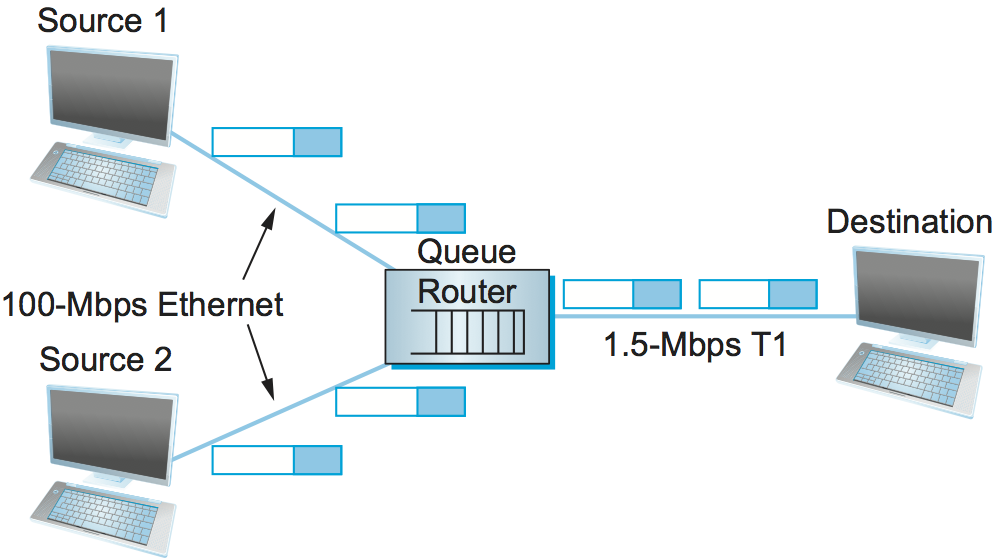
Figure 152. A potential bottleneck router.
We need to qualify the term connectionless because our classification of networks as being either connectionless or connection oriented is a bit too restrictive; there is a gray area in between. In particular, the assumption that all datagrams are completely independent in a connectionless network is too strong. The datagrams are certainly switched independently, but it is usually the case that a stream of datagrams between a particular pair of hosts flows through a particular set of routers. This idea of a flow—a sequence of packets sent between a source/destination pair and following the same route through the network—is an important abstraction in the context of resource allocation; it is one that we will use in this chapter.
One of the powers of the flow abstraction is that flows can be defined at different granularities. For example, a flow can be host-to-host (i.e., have the same source/destination host addresses) or process-to-process (i.e., have the same source/destination host/port pairs). In the latter case, a flow is essentially the same as a channel, as we have been using that term throughout this book. The reason we introduce a new term is that a flow is visible to the routers inside the network, whereas a channel is an end-to-end abstraction. Figure 153 illustrates several flows passing through a series of routers.
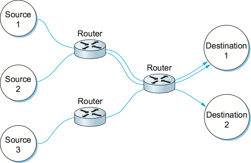
Figure 153. Multiple flows passing through a set of routers.
Because multiple related packets flow through each router, it sometimes makes sense to maintain some state information for each flow, information that can be used to make resource allocation decisions about the packets that belong to the flow. This state is sometimes called soft state. The main difference between soft state and hard state is that soft state need not always be explicitly created and removed by signalling. Soft state represents a middle ground between a purely connectionless network that maintains no state at the routers and a purely connection-oriented network that maintains hard state at the routers. In general, the correct operation of the network does not depend on soft state being present (each packet is still routed correctly without regard to this state), but when a packet happens to belong to a flow for which the router is currently maintaining soft state, then the router is better able to handle the packet.
Note that a flow can be either implicitly defined or explicitly established. In the former case, each router watches for packets that happen to be traveling between the same source/destination pair—the router does this by inspecting the addresses in the header—and treats these packets as belonging to the same flow for the purpose of congestion control. In the latter case, the source sends a flow setup message across the network, declaring that a flow of packets is about to start. While explicit flows are arguably no different than a connection across a connection-oriented network, we call attention to this case because, even when explicitly established, a flow does not imply any end-to-end semantics and, in particular, does not imply the reliable and ordered delivery of a virtual circuit. It simply exists for the purpose of resource allocation. We will see examples of both implicit and explicit flows in this chapter.
Service Model
In the early part of this chapter, we will focus on mechanisms that assume the best-effort service model of the Internet. With best-effort service, all packets are given essentially equal treatment, with end hosts given no opportunity to ask the network that some packets or flows be given certain guarantees or preferential service. Defining a service model that supports some kind of preferred service or guarantee—for example, guaranteeing the bandwidth needed for a video stream—is the subject of a later section. Such a service model is said to provide multiple qualities of service (QoS). As we will see, there is actually a spectrum of possibilities, ranging from a purely best-effort service model to one in which individual flows receive quantitative guarantees of QoS. One of the greatest challenges is to define a service model that meets the needs of a wide range of applications and even allows for the applications that will be invented in the future.
6.1.2 Taxonomy
There are countless ways in which resource allocation mechanisms differ, so creating a thorough taxonomy is a difficult proposition. For now, we describe three dimensions along which resource allocation mechanisms can be characterized; more subtle distinctions will be called out during the course of this chapter.
Router-Centric versus Host-Centric
Resource allocation mechanisms can be classified into two broad groups: those that address the problem from inside the network (i.e., at the routers or switches) and those that address it from the edges of the network (i.e., in the hosts, perhaps inside the transport protocol). Since it is the case that both the routers inside the network and the hosts at the edges of the network participate in resource allocation, the real issue is where the majority of the burden falls.
In a router-centric design, each router takes responsibility for deciding when packets are forwarded and selecting which packets are to be dropped, as well as for informing the hosts that are generating the network traffic how many packets they are allowed to send. In a host-centric design, the end hosts observe the network conditions (e.g., how many packets they are successfully getting through the network) and adjust their behavior accordingly. Note that these two groups are not mutually exclusive. For example, a network that places the primary burden for managing congestion on routers still expects the end hosts to adhere to any advisory messages the routers send, while the routers in networks that use end-to-end congestion control still have some policy, no matter how simple, for deciding which packets to drop when their queues do overflow.
Reservation-Based versus Feedback-Based
A second way that resource allocation mechanisms are sometimes classified is according to whether they use reservations or feedback. In a reservation-based system, some entity (e.g., the end host) asks the network for a certain amount of capacity to be allocated for a flow. Each router then allocates enough resources (buffers and/or percentage of the link’s bandwidth) to satisfy this request. If the request cannot be satisfied at some router, because doing so would overcommit its resources, then the router rejects the reservation. This is analogous to getting a busy signal when trying to make a phone call. In a feedback-based approach, the end hosts begin sending data without first reserving any capacity and then adjust their sending rate according to the feedback they receive. This feedback can be either explicit (i.e., a congested router sends a “please slow down” message to the host) or implicit (i.e., the end host adjusts its sending rate according to the externally observable behavior of the network, such as packet losses).
Note that a reservation-based system always implies a router-centric resource allocation mechanism. This is because each router is responsible for keeping track of how much of its capacity is currently available and deciding whether new reservations can be admitted. Routers may also have to make sure each host lives within the reservation it made. If a host sends data faster than it claimed it would when it made the reservation, then that host’s packets are good candidates for discarding, should the router become congested. On the other hand, a feedback-based system can imply either a router- or host-centric mechanism. Typically, if the feedback is explicit, then the router is involved, to at least some degree, in the resource allocation scheme. If the feedback is implicit, then almost all of the burden falls to the end host; the routers silently drop packets when they become congested.
Reservations do not have to be made by end hosts. It is possible for a network administrator to allocate resources to flows or to larger aggregates of traffic, as we will see in a later section.
Window Based versus Rate Based
A third way to characterize resource allocation mechanisms is according to whether they are window based or rate based. This is one of the areas, noted above, where similar mechanisms and terminology are used for both flow control and congestion control. Both flow-control and resource allocation mechanisms need a way to express, to the sender, how much data it is allowed to transmit. There are two general ways of doing this: with a window or with a rate. We have already seen window-based transport protocols, such as TCP, in which the receiver advertises a window to the sender. This window corresponds to how much buffer space the receiver has, and it limits how much data the sender can transmit; that is, it supports flow control. A similar mechanism—window advertisement—can be used within the network to reserve buffer space (i.e., to support resource allocation). TCP’s congestion-control mechanisms are window based.
It is also possible to control a sender’s behavior using a rate—that is, how many bits per second the receiver or network is able to absorb. Rate-based control makes sense for many multimedia applications, which tend to generate data at some average rate and which need at least some minimum throughput to be useful. For example, a video codec might generate video at an average rate of 1 Mbps with a peak rate of 2 Mbps. As we will see later in this chapter, rate-based characterization of flows is a logical choice in a reservation-based system that supports different qualities of service—the sender makes a reservation for so many bits per second, and each router along the path determines if it can support that rate, given the other flows it has made commitments to.
Summary of Resource Allocation Taxonomy
Classifying resource allocation approaches at two different points along each of three dimensions, as we have just done, would seem to suggest up to eight unique strategies. While eight different approaches are certainly possible, we note that in practice two general strategies seem to be most prevalent; these two strategies are tied to the underlying service model of the network.
On the one hand, a best-effort service model usually implies that feedback is being used, since such a model does not allow users to reserve network capacity. This, in turn, means that most of the responsibility for congestion control falls to the end hosts, perhaps with some assistance from the routers. In practice, such networks use window-based information. This is the general strategy adopted in the Internet.
On the other hand, a QoS-based service model probably implies some form of reservation. Support for these reservations is likely to require significant router involvement, such as queuing packets differently depending on the level of reserved resources they require. Moreover, it is natural to express such reservations in terms of rate, since windows are only indirectly related to how much bandwidth a user needs from the network. We discuss this topic in a later section.
6.1.3 Evaluation Criteria
The final issue is one of knowing whether a resource allocation mechanism is good or not. Recall that in the problem statement at the start of this chapter we posed the question of how a network effectively and fairly allocates its resources. This suggests at least two broad measures by which a resource allocation scheme can be evaluated. We consider each in turn.
Effective Resource Allocation
A good starting point for evaluating the effectiveness of a resource allocation scheme is to consider the two principal metrics of networking: throughput and delay. Clearly, we want as much throughput and as little delay as possible. Unfortunately, these goals are often somewhat at odds with each other. One sure way for a resource allocation algorithm to increase throughput is to allow as many packets into the network as possible, so as to drive the utilization of all the links up to 100%. We would do this to avoid the possibility of a link becoming idle because an idle link necessarily hurts throughput. The problem with this strategy is that increasing the number of packets in the network also increases the length of the queues at each router. Longer queues, in turn, mean packets are delayed longer in the network.
To describe this relationship, some network designers have proposed using the ratio of throughput to delay as a metric for evaluating the effectiveness of a resource allocation scheme. This ratio is sometimes referred to as the power of the network:
Power = Throughput / Delay
Note that it is not obvious that power is the right metric for judging resource allocation effectiveness. For one thing, the theory behind power is based on an M/M/1 queuing network that assumes infinite queues;1 real networks have finite buffers and sometimes have to drop packets. For another, power is typically defined relative to a single connection (flow); it is not clear how it extends to multiple, competing connections. Despite these rather severe limitations, however, no alternatives have gained wide acceptance, and so power continues to be used.
- 1
Since this is not a queuing theory book, we provide only this brief description of an M/M/1 queue. The 1 means it has a single server, and the Ms mean that the distribution of both packet arrival and service times is Markovian, that is, exponential.
The objective is to maximize this ratio, which is a function of how much load you place on the network. The load, in turn, is set by the resource allocation mechanism. Figure 154 gives a representative power curve, where, ideally, the resource allocation mechanism would operate at the peak of this curve. To the left of the peak, the mechanism is being too conservative; that is, it is not allowing enough packets to be sent to keep the links busy. To the right of the peak, so many packets are being allowed into the network that increases in delay due to queuing are starting to dominate any small gains in throughput.
Interestingly, this power curve looks very much like the system throughput curve in a timesharing computer system. System throughput improves as more jobs are admitted into the system, until it reaches a point when there are so many jobs running that the system begins to thrash (spends all of its time swapping memory pages) and the throughput begins to drop.
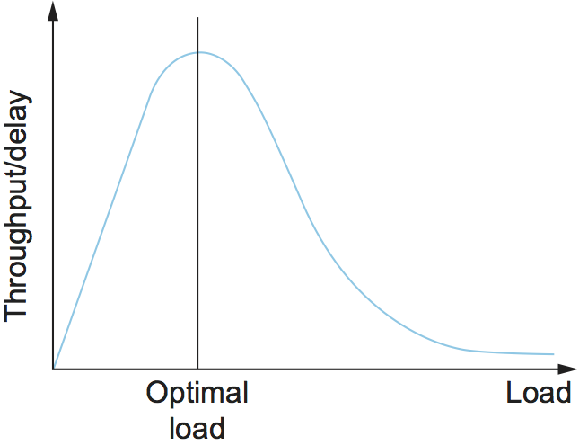
Figure 154. Ratio of throughput to delay as a function of load.
As we will see in later sections of this chapter, many congestion-control schemes are able to control load in only very crude ways; that is, it is simply not possible to turn the “knob” a little and allow only a small number of additional packets into the network. As a consequence, network designers need to be concerned about what happens even when the system is operating under extremely heavy load—that is, at the rightmost end of the curve in Figure 154. Ideally, we would like to avoid the situation in which the system throughput goes to zero because the system is thrashing. In networking terminology, we want a system that is stable—where packets continue to get through the network even when the network is operating under heavy load. If a mechanism is not stable, the network may experience congestion collapse.
Fair Resource Allocation
The effective utilization of network resources is not the only criterion for judging a resource allocation scheme. We must also consider the issue of fairness. However, we quickly get into murky waters when we try to define what exactly constitutes fair resource allocation. For example, a reservation-based resource allocation scheme provides an explicit way to create controlled unfairness. With such a scheme, we might use reservations to enable a video stream to receive 1 Mbps across some link while a file transfer receives only 10 kbps over the same link.
In the absence of explicit information to the contrary, when several flows share a particular link, we would like for each flow to receive an equal share of the bandwidth. This definition presumes that a fair share of bandwidth means an equal share of bandwidth. But, even in the absence of reservations, equal shares may not equate to fair shares. Should we also consider the length of the paths being compared? For example, as illustrated in Figure 155, what is fair when one four-hop flow is competing with three one-hop flows?
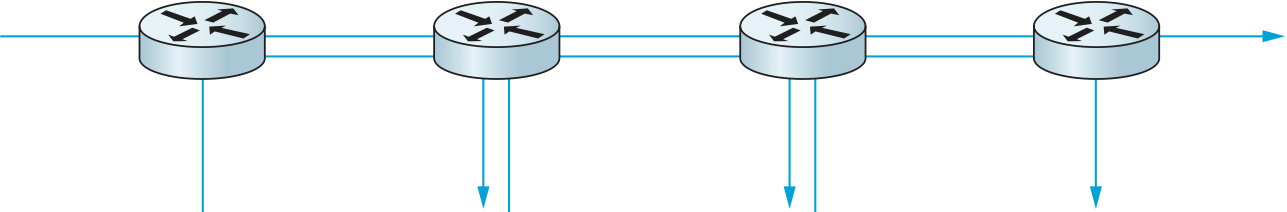
Figure 155. One four-hop flow competing with three one-hop flows.
Assuming that fair implies equal and that all paths are of equal length, networking researcher Raj Jain proposed a metric that can be used to quantify the fairness of a congestion-control mechanism. Jain’s fairness index is defined as follows. Given a set of flow throughputs
(measured in consistent units such as bits/second), the following function assigns a fairness index to the flows:
The fairness index always results in a number between 0 and 1, with 1 representing greatest fairness. To understand the intuition behind this metric, consider the case where all n flows receive a throughput of 1 unit of data per second. We can see that the fairness index in this case is
Now, suppose one flow receives a throughput of \(1 + \Delta\). Now the fairness index is
Note that the denominator exceeds the numerator by \((n-1)\Delta^2\). Thus, whether the odd flow out was getting more or less than all the other flows (positive or negative \(\Delta\)), the fairness index has now dropped below one. Another simple case to consider is where only k of the n flows receive equal throughput, and the remaining n-k users receive zero throughput, in which case the fairness index drops to k/n.