6.5 Quality of Service
The promise of general-purpose packet-switched networks is that they support all kinds of applications and data, including multimedia applications that transmit digitized audio and video streams. In the early days, one obstacle to the fulfillment of this promise was the need for higher-bandwidth links. That is no longer an issue, but there is more to transmitting audio and video over a network than just providing sufficient bandwidth.
Participants in a telephone conversation, for example, expect to be able to converse in such a way that one person can respond to something said by the other and be heard almost immediately. Thus, the timeliness of delivery can be very important. We refer to applications that are sensitive to the timeliness of data as real-time applications. Voice and video applications tend to be the canonical examples, but there are others such as industrial control—you would like a command sent to a robot arm to reach it before the arm crashes into something. Even file transfer applications can have timeliness constraints, such as a requirement that a database update complete overnight before the business that needs the data resumes on the next day.
The distinguishing characteristic of real-time applications is that they need some sort of assurance from the network that data is likely to arrive on time (for some definition of “on time”). Whereas a non-real-time application can use an end-to-end retransmission strategy to make sure that data arrives correctly, such a strategy cannot provide timeliness: Retransmission only adds to total latency if data arrives late. Timely arrival must be provided by the network itself (the routers), not just at the network edges (the hosts). We therefore conclude that the best-effort model, in which the network tries to deliver your data but makes no promises and leaves the cleanup operation to the edges, is not sufficient for real-time applications. What we need is a new service model, in which applications that need higher assurances can ask the network for them. The network may then respond by providing an assurance that it will do better or perhaps by saying that it cannot promise anything better at the moment. Note that such a service model is a superset of the original model: Applications that are happy with best-effort service should be able to use the new service model; their requirements are just less stringent. This implies that the network will treat some packets differently from others—something that is not done in the best-effort model. A network that can provide these different levels of service is often said to support quality of service (QoS).
6.5.1 Application Requirements
Before looking at the various protocols and mechanisms that may be used to provide quality of service to applications, we should try to understand what the needs of those applications are. To begin, we can divide applications into two types: real-time and non-real-time. The latter are sometimes called traditional data applications, since they have traditionally been the major applications found on data networks. They include most popular applications like SSH, file transfer, email, web browsing, and so on. All of these applications can work without guarantees of timely delivery of data. Another term for this non-real-time class of applications is elastic, since they are able to stretch gracefully in the face of increased delay. Note that these applications can benefit from shorter-length delays, but they do not become unusable as delays increase. Also note that their delay requirements vary from the interactive applications like SSH to more asynchronous ones like email, with interactive bulk transfers like file transfer in the middle.
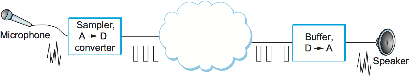
Figure 172. An audio application.
Real-Time Audio Example
As a concrete example of a real-time application, consider an audio application similar to the one illustrated in Figure 172. Data is generated by collecting samples from a microphone and digitizing them using an analog-to-digital (A-to-D) converter. The digital samples are placed in packets, which are transmitted across the network and received at the other end. At the receiving host, the data must be played back at some appropriate rate. For example, if the voice samples were collected at a rate of one per 125 μs, they should be played back at the same rate. Thus, we can think of each sample as having a particular playback time: the point in time at which it is needed in the receiving host. In the voice example, each sample has a playback time that is 125 μs later than the preceding sample. If data arrives after its appropriate playback time, either because it was delayed in the network or because it was dropped and subsequently retransmitted, it is essentially useless. It is the complete worthlessness of late data that characterizes real-time applications. In elastic applications, it might be nice if data turns up on time, but we can still use it when it does not.
One way to make our voice application work would be to make sure all samples take exactly the same amount of time to traverse the network. Then, since samples are injected at a rate of one per 125 μs, they will appear at the receiver at the same rate, ready to be played back. However, it is generally difficult to guarantee that all data traversing a packet-switched network will experience exactly the same delay. Packets encounter queues in switches or routers, and the lengths of these queues vary with time, meaning that the delays tend to vary with time and, as a consequence, are potentially different for each packet in the audio stream. The way to deal with this at the receiver end is to buffer up some amount of data in reserve, thereby always providing a store of packets waiting to be played back at the right time. If a packet is delayed a short time, it goes in the buffer until its playback time arrives. If it gets delayed a long time, then it will not need to be stored for very long in the receiver’s buffer before being played back. Thus, we have effectively added a constant offset to the playback time of all packets as a form of insurance. We call this offset the playback point. The only time we run into trouble is if packets get delayed in the network for such a long time that they arrive after their playback time, causing the playback buffer to be drained.
The operation of a playback buffer is illustrated in Figure 173. The left-hand diagonal line shows packets being generated at a steady rate. The wavy line shows when the packets arrive, some variable amount of time after they were sent, depending on what they encountered in the network. The right-hand diagonal line shows the packets being played back at a steady rate, after sitting in the playback buffer for some period of time. As long as the playback line is far enough to the right in time, the variation in network delay is never noticed by the application. However, if we move the playback line a little to the left, then some packets will begin to arrive too late to be useful.
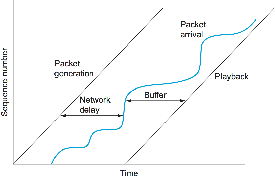
Figure 173. A playback buffer.
For our audio application, there are limits to how far we can delay playing back data. It is hard to carry on a conversation if the time between when you speak and when your listener hears you is more than 300 ms. Thus, what we want from the network in this case is a guarantee that all our data will arrive within 300 ms. If data arrives early, we buffer it until its correct playback time. If it arrives late, we have no use for it and must discard it.
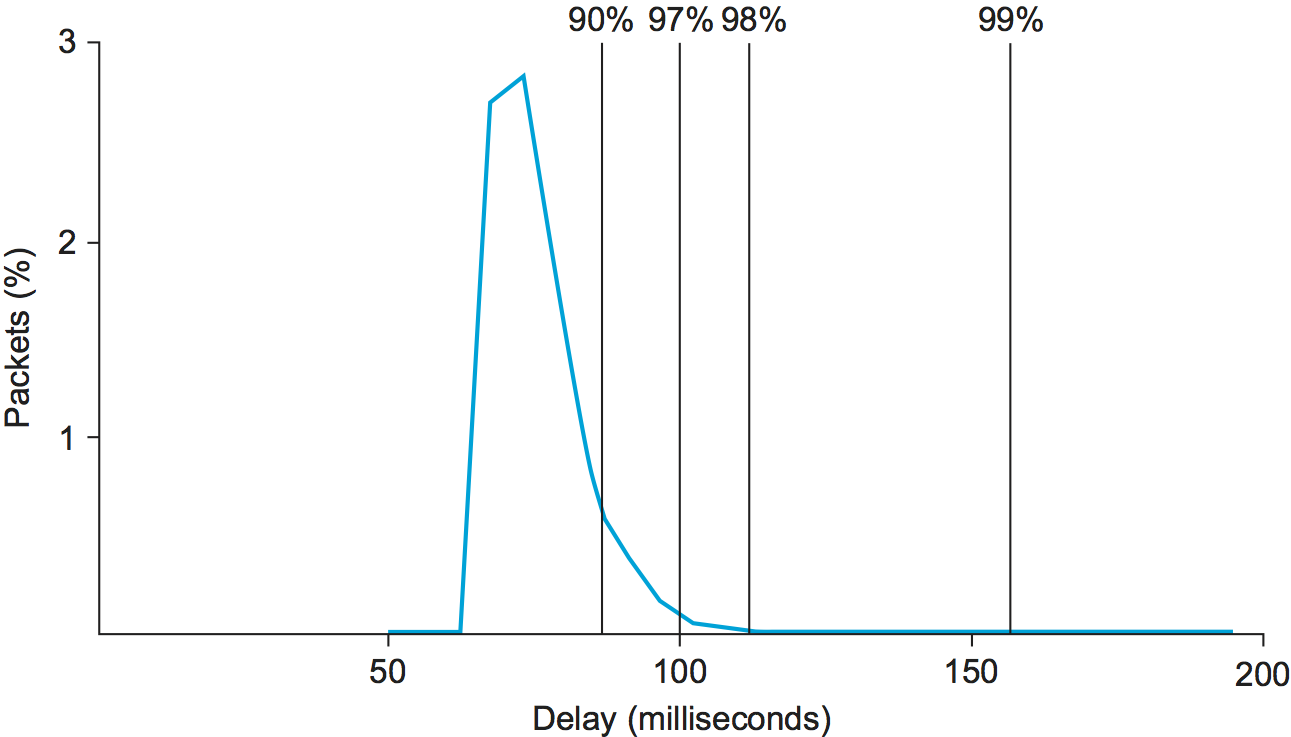
Figure 174. Example distribution of delays for an Internet connection.
To get a better appreciation of how variable network delay can be, Figure 174 shows the one-way delay measured over a certain path across the Internet over the course of one particular day. While the exact numbers would vary depending on the path and the date, the key factor here is the variability of the delay, which is consistently found on almost any path at any time. As denoted by the cumulative percentages given across the top of the graph, 97% of the packets in this case had a latency of 100 ms or less. This means that if our example audio application were to set the playback point at 100 ms, then, on average, 3 out of every 100 packets would arrive too late to be of any use. One important thing to notice about this graph is that the tail of the curve—how far it extends to the right—is very long. We would have to set the playback point at over 200 ms to ensure that all packets arrived in time.
Taxonomy of Real-Time Applications
Now that we have a concrete idea of how real-time applications work, we can look at some different classes of applications that serve to motivate our service model. The following taxonomy owes much to the work of Clark, Braden, Shenker, and Zhang, whose papers on this subject can be found in the Further Reading section for this chapter. The taxonomy of applications is summarized in Figure 175.
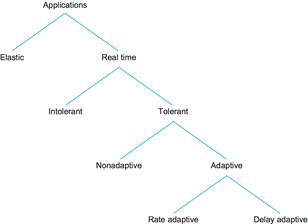
Figure 175. Taxonomy of applications.
The first characteristic by which we can categorize applications is their tolerance of loss of data, where “loss” might occur because a packet arrived too late to be played back as well as arising from the usual causes in the network. On the one hand, one lost audio sample can be interpolated from the surrounding samples with relatively little effect on the perceived audio quality. It is only as more and more samples are lost that quality declines to the point that the speech becomes incomprehensible. On the other hand, a robot control program is likely to be an example of a real-time application that cannot tolerate loss—losing the packet that contains the command instructing the robot arm to stop is unacceptable. Thus, we can categorize real-time applications as tolerant or intolerant depending on whether they can tolerate occasional loss. (As an aside, note that many real-time applications are more tolerant of occasional loss than non-real-time applications; for example, compare our audio application to file transfer, where the uncorrected loss of one bit might render a file completely useless.)
A second way to characterize real-time applications is by their
adaptability. For example, an audio application might be able to adapt
to the amount of delay that packets experience as they traverse the
network. If we notice that packets are almost always arriving within
300 ms of being sent, then we can set our playback point accordingly,
buffering any packets that arrive in less than 300 ms. Suppose that we
subsequently observe that all packets are arriving within 100 ms of
being sent. If we moved up our playback point to 100 ms, then the users
of the application would probably perceive an improvement. The process
of shifting the playback point would actually require us to play out
samples at an increased rate for some period of time. With a voice
application, this can be done in a way that is barely perceptible,
simply by shortening the silences between words. Thus, playback point
adjustment is fairly easy in this case, and it has been effectively
implemented for several voice applications such as the audio
teleconferencing program known as vat. Note that playback point
adjustment can happen in either direction, but that doing so actually
involves distorting the played-back signal during the period of
adjustment, and that the effects of this distortion will very much
depend on how the end user uses the data.
Observe that if we set our playback point on the assumption that all packets will arrive within 100 ms and then find that some packets are arriving slightly late, we will have to drop them, whereas we would not have had to drop them if we had left the playback point at 300 ms. Thus, we should advance the playback point only when it provides a perceptible advantage and only when we have some evidence that the number of late packets will be acceptably small. We may do this because of observed recent history or because of some assurance from the network.
We call applications that can adjust their playback point delay-adaptive applications. Another class of adaptive applications is rate adaptive. For example, many video coding algorithms can trade off bit rate versus quality. Thus, if we find that the network can support a certain bandwidth, we can set our coding parameters accordingly. If more bandwidth becomes available later, we can change parameters to increase the quality.
Approaches to QoS Support
Considering this rich space of application requirements, what we need is a richer service model that meets the needs of any application. This leads us to a service model with not just one class (best effort), but with several classes, each available to meet the needs of some set of applications. Towards this end, we are now ready to look at some of the approaches that have been developed to provide a range of qualities of service. These can be divided into two broad categories:
Fine-grained approaches, which provide QoS to individual applications or flows
Coarse-grained approaches, which provide QoS to large classes of data or aggregated traffic
In the first category, we find Integrated Services, a QoS architecture developed in the IETF and often associated with the Resource Reservation Protocol (RSVP). In the second category lies Differentiated Services, which is probably the most widely deployed QoS mechanism today. We discuss these in turn in the next two subsections.
Finally, as we suggested at the start of this section, adding QoS support to the network isn’t necessarily the entire story about supporting real-time applications. We conclude our discussion by revisiting what the end-host might do to better support real-time streams, independent of how widely deployed QoS mechanisms like Integrated or Differentiated Services become.
6.5.2 Integrated Services (RSVP)
The term Integrated Services (often called IntServ for short) refers to a body of work that was produced by the IETF around 1995-97. The IntServ working group developed specifications of a number of service classes designed to meet the needs of some of the application types described above. It also defined how RSVP could be used to make reservations using these service classes. The following paragraphs provide an overview of these specifications and the mechanisms that are used to implement them.
Service Classes
One of the service classes is designed for intolerant applications. These applications require that a packet never arrive late. The network should guarantee that the maximum delay that any packet will experience has some specified value; the application can then set its playback point so that no packet will ever arrive after its playback time. We assume that early arrival of packets can always be handled by buffering. This service is referred to as the guaranteed service.
In addition to the guaranteed service, the IETF considered several other services, but eventually settled on one to meet the needs of tolerant, adaptive applications. The service is known as controlled load and was motivated by the observation that existing applications of this type run quite well on networks that are not heavily loaded. Audio applications, for example, adjust their playback point as network delay varies and produces reasonable audio quality as long as loss rates remain on the order of 10% or less.
The aim of the controlled load service is to emulate a lightly loaded network for those applications that request the service, even though the network as a whole may in fact be heavily loaded. The trick to this is to use a queuing mechanism such as WFQ to isolate the controlled load traffic from the other traffic and some form of admission control to limit the total amount of controlled load traffic on a link such that the load is kept reasonably low. We discuss admission control in more detail below.
Clearly, these two service classes are a subset of all the classes that might be provided. In fact, other services were specified but never standardized as part of the IETF’s work. So far, the two services described above (along with traditional best effort) have proven flexible enough to meet the needs of a wide range of applications.
Overview of Mechanisms
Now that we have augmented our best-effort service model with some new service classes, the next question is how we implement a network that provides these services to applications. This section outlines the key mechanisms. Keep in mind while reading this section that the mechanisms being described are still being hammered out by the Internet design community. The main thing to take away from the discussion is a general understanding of the pieces involved in supporting the service model outlined above.
First, whereas with a best-effort service we can just tell the network where we want our packets to go and leave it at that, a real-time service involves telling the network something more about the type of service we require. We may give it qualitative information such as “use a controlled load service” or quantitative information such as “I need a maximum delay of 100 ms.” In addition to describing what we want, we need to tell the network something about what we are going to inject into it, since a low-bandwidth application is going to require fewer network resources than a high-bandwidth application. The set of information that we provide to the network is referred to as a flowspec. This name comes from the idea that a set of packets associated with a single application and that share common requirements is called a flow, consistent with our use of the term in the earlier section outlining the relevant issues.
Second, when we ask the network to provide us with a particular service, the network needs to decide if it can in fact provide that service. For example, if 10 users ask for a service in which each will consistently use 2 Mbps of link capacity, and they all share a link with 10-Mbps capacity, the network will have to say no to some of them. The process of deciding when to say no is called admission control.
Third, we need a mechanism by which the users of the network and the components of the network itself exchange information such as requests for service, flowspecs, and admission control decisions. This is sometimes called signalling, but since that word has several meanings, we refer to this process as resource reservation, and it is achieved using a resource reservation protocol.
Finally, when flows and their requirements have been described, and admission control decisions have been made, the network switches and routers need to meet the requirements of the flows. A key part of meeting these requirements is managing the way packets are queued and scheduled for transmission in the switches and routers. This last mechanism is packet scheduling.
Flowspecs
There are two separable parts to the flowspec: the part that describes the flow’s traffic characteristics (called the TSpec) and the part that describes the service requested from the network (the RSpec). The RSpec is very service specific and relatively easy to describe. For example, with a controlled load service, the RSpec is trivial: The application just requests controlled load service with no additional parameters. With a guaranteed service, you could specify a delay target or bound. (In the IETF’s guaranteed service specification, you specify not a delay but another quantity from which delay can be calculated.)
The TSpec is a little more complicated. As our example above showed, we need to give the network enough information about the bandwidth used by the flow to allow intelligent admission control decisions to be made. For most applications, however, the bandwidth is not a single number; it is something that varies constantly. A video application, for example, will generally generate more bits per second when the scene is changing rapidly than when it is still. Just knowing the long-term average bandwidth is not enough, as the following example illustrates. Suppose that we have 10 flows that arrive at a switch on separate input ports and that all leave on the same 10-Mbps link. Assume that over some suitably long interval each flow can be expected to send no more than 1 Mbps. You might think that this presents no problem. However, if these are variable bit rate applications, such as compressed video, then they will occasionally send more than their average rates. If enough sources send at above their average rates, then the total rate at which data arrives at the switch will be greater than 10 Mbps. This excess data will be queued before it can be sent on the link. The longer this condition persists, the longer the queue will get. Packets might have to be dropped and, even if it doesn’t come to that, data sitting in the queue is being delayed. If packets are delayed long enough, the service that was requested will not be provided.
Exactly how we manage our queues to control delay and avoid dropping packets is something we discuss below. However, note here that we need to know something about how the bandwidth of our sources varies with time. One way to describe the bandwidth characteristics of sources is called a token bucket filter. Such a filter is described by two parameters: a token rate r, and a bucket depth B. It works as follows. To be able to send a byte, I must have a token. To send a packet of length n, I need n tokens. I start with no tokens and I accumulate them at a rate of r per second. I can accumulate no more than B tokens. What this means is that I can send a burst of as many as B bytes into the network as fast as I want, but over a sufficiently long interval I can’t send more than r bytes per second. It turns out that this information is very helpful to the admission control algorithm when it tries to figure out whether it can accommodate a new request for service.
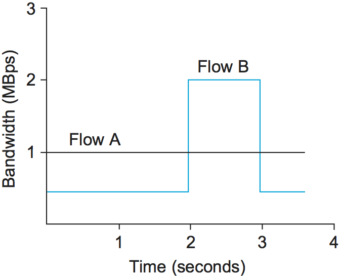
Figure 176. Two flows with equal average rates but different token bucket descriptions.
Figure 176 illustrates how a token bucket can be used to characterize a flow’s bandwidth requirements. For simplicity, assume that each flow can send data as individual bytes rather than as packets. Flow A generates data at a steady rate of 1 MBps, so it can be described by a token bucket filter with a rate r = 1 MBps and a bucket depth of 1 byte. This means that it receives tokens at a rate of 1 MBps but that it cannot store more than 1 token—it spends them immediately. Flow B also sends at a rate that averages out to 1 MBps over the long term, but does so by sending at 0.5 MBps for 2 seconds and then at 2 MBps for 1 second. Since the token bucket rate r is, in a sense, a long-term average rate, flow B can be described by a token bucket with a rate of 1 MBps. Unlike flow A, however, flow B needs a bucket depth B of at least 1 MB, so that it can store up tokens while it sends at less than 1 MBps to be used when it sends at 2 MBps. For the first 2 seconds in this example, it receives tokens at a rate of 1 MBps but spends them at only 0.5 MBps, so it can save up 2 × 0.5 = 1 MB of tokens, which it then spends in the third second (along with the new tokens that continue to accrue in that second) to send data at 2 MBps. At the end of the third second, having spent the excess tokens, it starts to save them up again by sending at 0.5 MBps again.
It is interesting to note that a single flow can be described by many different token buckets. As a trivial example, flow A could be described by the same token bucket as flow B, with a rate of 1 MBps and a bucket depth of 1 MB. The fact that it never actually needs to accumulate tokens does not make that an inaccurate description, but it does mean that we have failed to convey some useful information to the network—the fact that flow A is actually very consistent in its bandwidth needs. In general, it is good to be as explicit about the bandwidth needs of an application as possible to avoid over-allocation of resources in the network.
Admission Control
The idea behind admission control is simple: When some new flow wants to receive a particular level of service, admission control looks at the TSpec and RSpec of the flow and tries to decide if the desired service can be provided to that amount of traffic, given the currently available resources, without causing any previously admitted flow to receive worse service than it had requested. If it can provide the service, the flow is admitted; if not, then it is denied. The hard part is figuring out when to say yes and when to say no.
Admission control is very dependent on the type of requested service and on the queuing discipline employed in the routers; we discuss the latter topic later in this section. For a guaranteed service, you need to have a good algorithm to make a definitive yes/no decision. The decision is fairly straightforward if weighted fair queuing is used at each router. For a controlled load service, the decision may be based on heuristics, such as “The last time I allowed a flow with this TSpec into this class, the delays for the class exceeded the acceptable bound, so I’d better say no” or “My current delays are so far inside the bounds that I should be able to admit another flow without difficulty.”
Admission control should not be confused with policing. The former is a per-flow decision to admit a new flow or not. The latter is a function applied on a per-packet basis to make sure that a flow conforms to the TSpec that was used to make the reservation. If a flow does not conform to its TSpec—for example, because it is sending twice as many bytes per second as it said it would—then it is likely to interfere with the service provided to other flows, and some corrective action must be taken. There are several options, the obvious one being to drop offending packets. However, another option would be to check if the packets really are interfering with the service of other flows. If they are not interfering, the packets could be sent on after being marked with a tag that says, in effect, “This is a nonconforming packet. Drop it first if you need to drop any packets.”
Admission control is closely related to the important issue of policy. For example, a network administrator might wish to allow reservations made by his company’s CEO to be admitted while rejecting reservations made by more lowly employees. Of course, the CEO’s reservation request might still fail if the requested resources aren’t available, so we see that issues of policy and resource availability may both be addressed when admission control decisions are made. The application of policy to networking is an area receiving much attention at the time of writing.
Reservation Protocol
While connection-oriented networks have always needed some sort of setup protocol to establish the necessary virtual circuit state in the switches, connectionless networks like the Internet have had no such protocols. As this section has indicated, however, we need to provide a lot more information to our network when we want a real-time service from it. While there have been a number of setup protocols proposed for the Internet, the one on which most current attention is focused is the RSVP. It is particularly interesting because it differs so substantially from conventional signalling protocols for connection-oriented networks.
One of the key assumptions underlying RSVP is that it should not detract from the robustness that we find in today’s connectionless networks. Because connectionless networks rely on little or no state being stored in the network itself, it is possible for routers to crash and reboot and for links to go up and down while end-to-end connectivity is still maintained. RSVP tries to maintain this robustness by using the idea of soft state in the routers. Soft state—in contrast to the hard state found in connection-oriented networks—does not need to be explicitly deleted when it is no longer needed. Instead, it times out after some fairly short period (say, a minute) if it is not periodically refreshed. We will see later how this helps robustness.
Another important characteristic of RSVP is that it aims to support multicast flows just as effectively as unicast flows. This is not surprising, since many of the first applications that could benefit from improved quality of service were also multicast applications—video conferencing tools, for example. One of the insights of RSVP’s designers is that most multicast applications have many more receivers than senders, as typified by the large audience and one speaker for a lecture. Also, receivers may have different requirements. For example, one receiver might want to receive data from only one sender, while others might wish to receive data from all senders. Rather than having the senders keep track of a potentially large number of receivers, it makes more sense to let the receivers keep track of their own needs. This suggests the receiver-oriented approach adopted by RSVP. In contrast, connection-oriented networks usually leave resource reservation to the sender, just as it is normally the originator of a phone call who causes resources to be allocated in the phone network.
The soft state and receiver-oriented nature of RSVP give it a number of good properties. One such property is that it is very straightforward to increase or decrease the level of resource allocation provided to a receiver. Since each receiver periodically sends refresh messages to keep the soft state in place, it is easy to send a new reservation that asks for a new level of resources. Further, soft state deals gracefully with the possibility of network or node failures. In the event of a host crash, resources allocated by that host to a flow will naturally time out and be released. To see what happens in the event of a router or link failure, we need to look a little more closely at the mechanics of making a reservation.
Initially, consider the case of one sender and one receiver trying to get a reservation for traffic flowing between them. There are two things that need to happen before a receiver can make the reservation. First, the receiver needs to know what traffic the sender is likely to send so that it can make an appropriate reservation. That is, it needs to know the sender’s TSpec. Second, it needs to know what path the packets will follow from sender to receiver, so that it can establish a resource reservation at each router on the path. Both of these requirements can be met by sending a message from the sender to the receiver that contains the TSpec. Obviously, this gets the TSpec to the receiver. The other thing that happens is that each router looks at this message (called a PATH message) as it goes past, and it figures out the reverse path that will be used to send reservations from the receiver back to the sender in an effort to get the reservation to each router on the path. Building the multicast tree in the first place is done by mechanisms such as those described in another chapter.
Having received a PATH message, the receiver sends a reservation back up the multicast tree in a RESV message. This message contains the sender’s TSpec and an RSpec describing the requirements of this receiver. Each router on the path looks at the reservation request and tries to allocate the necessary resources to satisfy it. If the reservation can be made, the RESV request is passed on to the next router. If not, an error message is returned to the receiver who made the request. If all goes well, the correct reservation is installed at every router between the sender and the receiver. As long as the receiver wants to retain the reservation, it sends the same RESV message about once every 30 seconds.
Now we can see what happens when a router or link fails. Routing protocols will adapt to the failure and create a new path from sender to receiver. PATH messages are sent about every 30 seconds, and may be sent sooner if a router detects a change in its forwarding table, so the first one after the new route stabilizes will reach the receiver over the new path. The receiver’s next RESV message will follow the new path and, if all goes well, establish a new reservation on the new path. Meanwhile, the routers that are no longer on the path will stop getting RESV messages, and these reservations will time out and be released. Thus, RSVP deals quite well with changes in topology, as long as routing changes are not excessively frequent.
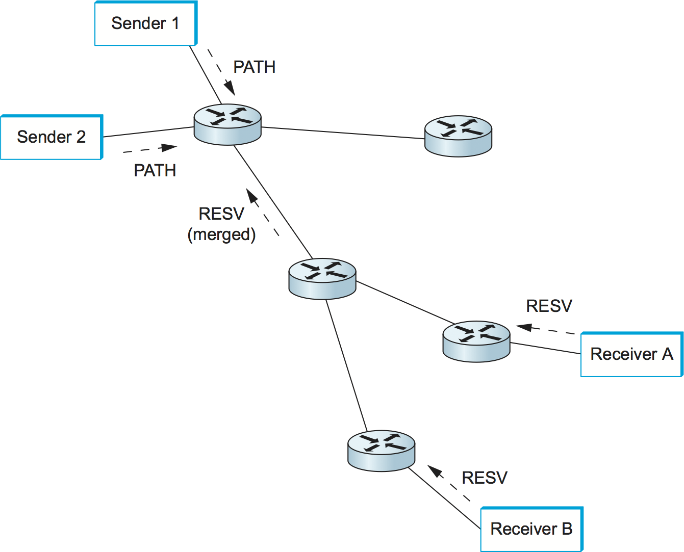
Figure 177. Making reservations on a multicast tree.
The next thing we need to consider is how to cope with multicast, where there may be multiple senders to a group and multiple receivers. This situation is illustrated in Figure 177. First, let’s deal with multiple receivers for a single sender. As a RESV message travels up the multicast tree, it is likely to hit a piece of the tree where some other receiver’s reservation has already been established. It may be the case that the resources reserved upstream of this point are adequate to serve both receivers. For example, if receiver A has already made a reservation that provides for a guaranteed delay of less than 100 ms, and the new request from receiver B is for a delay of less than 200 ms, then no new reservation is required. On the other hand, if the new request were for a delay of less than 50 ms, then the router would first need to see if it could accept the request; if so, it would send the request on upstream. The next time receiver A asked for a minimum of a 100-ms delay, the router would not need to pass this request on. In general, reservations can be merged in this way to meet the needs of all receivers downstream of the merge point.
If there are also multiple senders in the tree, receivers need to collect the TSpecs from all senders and make a reservation that is large enough to accommodate the traffic from all senders. However, this may not mean that the TSpecs need to be added up. For example, in an audioconference with 10 speakers, there is not much point in allocating enough resources to carry 10 audio streams, since the result of 10 people speaking at once would be incomprehensible. Thus, we could imagine a reservation that is large enough to accommodate two speakers and no more. Calculating the correct overall TSpec from all of the sender TSpecs is clearly application specific. Also, we may only be interested in hearing from a subset of all possible speakers; RSVP has different reservation styles to deal with such options as “Reserve resources for all speakers,” “Reserve resources for any \(n\) speakers,” and “Reserve resources for speakers A and B only.”
Packet Classifying and Scheduling
Once we have described our traffic and our desired network service and have installed a suitable reservation at all the routers on the path, the only thing that remains is for the routers to actually deliver the requested service to the data packets. There are two things that need to be done:
Associate each packet with the appropriate reservation so that it can be handled correctly, a process known as classifying packets.
Manage the packets in the queues so that they receive the service that has been requested, a process known as packet scheduling.
The first part is done by examining up to five fields in the packet: the
source address, destination address, protocol number, source port, and
destination port. (In IPv6, it is possible that the FlowLabel field
in the header could be used to enable the lookup to be done based on a
single, shorter key.) Based on this information, the packet can be
placed in the appropriate class. For example, it may be classified into
the controlled load classes, or it may be part of a guaranteed flow that
needs to be handled separately from all other guaranteed flows. In
short, there is a mapping from the flow-specific information in the
packet header to a single class identifier that determines how the
packet is handled in the queue. For guaranteed flows this might be a
one-to-one mapping, while for other services it might be many to one.
The details of classification are closely related to the details of
queue management.
It should be clear that something as simple as a FIFO queue in a router will be inadequate to provide many different services and to provide different levels of delay within each service. Several more sophisticated queue management disciplines were discussed in an earlier section, and some combination of these is likely to be used in a router.
The details of packet scheduling ideally should not be specified in the service model. Instead, this is an area where implementors can try to do creative things to realize the service model efficiently. In the case of guaranteed service, it has been established that a weighted fair queuing discipline, in which each flow gets its own individual queue with a certain share of the link, will provide a guaranteed end-to-end delay bound that can readily be calculated. For controlled load, simpler schemes may be used. One possibility includes treating all the controlled load traffic as a single, aggregated flow (as far as the scheduling mechanism is concerned), with the weight for that flow being set based on the total amount of traffic admitted in the controlled load class. The problem is made harder when you consider that, in a single router, many different services are likely to be provided concurrently and that each of these services may require a different scheduling algorithm. Thus, some overall queue management algorithm is needed to manage the resources between the different services.
Scalability Issues
Although the Integrated Services architecture and RSVP represented a significant enhancement of the best-effort service model of IP, many Internet service providers felt that it was not the right model for them to deploy. The reason for this reticence relates to one of the fundamental design goals of IP: scalability. In the best-effort service model, routers in the Internet store little or no state about the individual flows passing through them. Thus, as the Internet grows, the only thing routers have to do to keep up with that growth is to move more bits per second and to deal with larger routing tables, but RSVP raises the possibility that every flow passing through a router might have a corresponding reservation. To understand the severity of this problem, suppose that every flow on an OC-48 (2.5-Gbps) link represents a 64-kbps audio stream. The number of such flows is
2.5 × 10⁹ / 64 × 103 = 39,000
Each of those reservations needs some amount of state that needs to be stored in memory and refreshed periodically. The router needs to classify, police, and queue each of those flows. Admission control decisions need to be made every time such a flow requests a reservation, and some mechanism is needed to “push back” on users (e.g., charge their credit cards) so that they don’t make arbitrarily large reservations for long periods of time.
These scalability concerns have limited widespread deployment of IntServ. Because of these concerns, other approaches that do not require so much “per-flow” state have been developed. The next section discusses a number of such approaches.
6.5.3 Differentiated Services (EF, AF)
Whereas the Integrated Services architecture allocates resources to individual flows, the Differentiated Services model (often called DiffServ for short) allocates resources to a small number of classes of traffic. In fact, some proposed approaches to DiffServ simply divide traffic into two classes. This is an eminently sensible approach to take: If you consider the difficulty that network operators experience just trying to keep a best-effort internet running smoothly, it makes sense to add to the service model in small increments.
Suppose that we have decided to enhance the best-effort service model by adding just one new class, which we’ll call “premium.” Clearly, we will need some way to figure out which packets are premium and which are regular old best effort. Rather than using a protocol like RSVP to tell all the routers that some flow is sending premium packets, it would be much easier if the packets could just identify themselves to the router when they arrive. This could obviously be done by using a bit in the packet header—if that bit is a 1, the packet is a premium packet; if it’s a 0, the packet is best effort. With this in mind, there are two questions we need to address:
Who sets the premium bit and under what circumstances?
What does a router do differently when it sees a packet with the bit set?
There are many possible answers to the first question, but a common approach is to set the bit at an administrative boundary. For example, the router at the edge of an Internet service provider’s network might set the bit for packets arriving on an interface that connects to a particular company’s network. The Internet service provider might do this because that company has paid for a higher level of service than best effort. It is also possible that not all packets would be marked as premium; for example, the router might be configured to mark packets as premium up to some maximum rate and to leave all excess packets as best effort.
Assuming that packets have been marked in some way, what do the routers
that encounter marked packets do with them? Here again there are many
answers. In fact, the IETF standardized a set of router behaviors to be
applied to marked packets. These are called per-hop behaviors (PHBs),
a term that indicates that they define the behavior of individual
routers rather than end-to-end services. Because there is more than one
new behavior, there is also a need for more than 1 bit in the packet
header to tell the routers which behavior to apply. The IETF decided to
take the old TOS byte from the IP header, which had not been widely
used, and redefine it. Six bits of this byte have been allocated for
DiffServ code points (DSCPs), where each DSCP is a 6-bit value that
identifies a particular PHB to be applied to a packet. (The remaining
two bits are used by ECN.)
The Expedited Forwarding (EF) PHB
One of the simplest PHBs to explain is known as expedited forwarding (EF). Packets marked for EF treatment should be forwarded by the router with minimal delay and loss. The only way that a router can guarantee this to all EF packets is if the arrival rate of EF packets at the router is strictly limited to be less than the rate at which the router can forward EF packets. For example, a router with a 100-Mbps interface needs to be sure that the arrival rate of EF packets destined for that interface never exceeds 100 Mbps. It might also want to be sure that the rate will be somewhat below 100 Mbps, so that it occasionally has time to send other packets such as routing updates.
The rate limiting of EF packets is achieved by configuring the routers at the edge of an administrative domain to allow a certain maximum rate of EF packet arrivals into the domain. A simple, albeit conservative, approach would be to ensure that the sum of the rates of all EF packets entering the domain is less than the bandwidth of the slowest link in the domain. This would ensure that, even in the worst case where all EF packets converge on the slowest link, it is not overloaded and can provide the correct behavior.
There are several possible implementation strategies for the EF behavior. One is to give EF packets strict priority over all other packets. Another is to perform weighted fair queuing between EF packets and other packets, with the weight of EF set sufficiently high that all EF packets can be delivered quickly. This has an advantage over strict priority: The non-EF packets can be assured of getting some access to the link, even if the amount of EF traffic is excessive. This might mean that the EF packets fail to get exactly the specified behavior, but it could also prevent essential routing traffic from being locked out of the network in the event of an excessive load of EF traffic.
The Assured Forwarding (AF) PHB
The assured forwarding (AF) PHB has its roots in an approach known
as RED with In and Out (RIO) or Weighted RED, both of which are
enhancements to the basic RED algorithm described in an earlier
section. Figure 178 shows how RIO works; as
with RED, we see drop probability on the \(y\)-axis increasing as
average queue length increases along the \(x\)-axis. But now, for
our two classes of traffic, we have two separate drop probability
curves. RIO calls the two classes “in” and “out” for reasons that
will become clear shortly. Because the “out” curve has a lower
MinThreshold than the “in” curve, it is clear that, under low
levels of congestion, only packets marked “out” will be discarded by
the RED algorithm. If the congestion becomes more serious, a higher
percentage of “out” packets are dropped, and then if the average queue
length exceeds Minin, RED starts to drop “in” packets as well.
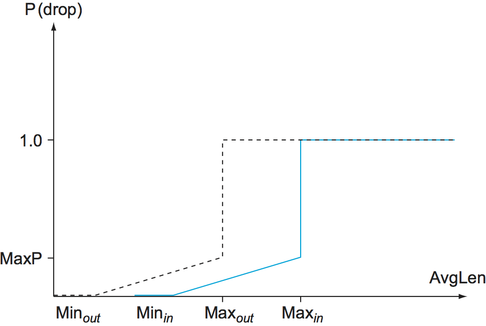
Figure 178. RED with In and Out drop probabilities.
The reason for calling the two classes of packets “in” and “out” stems from the way the packets are marked. We already noted that packet marking can be performed by a router at the edge of an administrative domain. We can think of this router as being at the boundary between a network service provider and some customer of that network. The customer might be any other network—for example, the network of a corporation or of another network service provider. The customer and the network service provider agree on some sort of profile for the assured service (and perhaps the customer pays the network service provider for this profile). The profile might be something like “Customer X is allowed to send up to \(y\) Mbps of assured traffic,” or it could be significantly more complex. Whatever the profile is, the edge router can clearly mark the packets that arrive from this customer as being either in or out of profile. In the example just mentioned, as long as the customer sends less than \(y\) Mbps, all his packets will be marked “in,” but once he exceeds that rate the excess packets will be marked “out.”
The combination of a profile meter at the edge and RIO in all the routers of the service provider’s network should provide the customer with a high assurance (but not a guarantee) that packets within his profile can be delivered. In particular, if the majority of packets, including those sent by customers who have not paid extra to establish a profile, are “out” packets, then it should usually be the case that the RIO mechanism will act to keep congestion low enough that “in” packets are rarely dropped. Clearly, there must be enough bandwidth in the network so that the “in” packets alone are rarely able to congest a link to the point where RIO starts dropping “in” packets.
Just like RED, the effectiveness of a mechanism like RIO depends to some extent on correct parameter choices, and there are considerably more parameters to set for RIO. Exactly how well the scheme will work in production networks is not known at the time of writing.
One interesting property of RIO is that it does not change the order of “in” and “out” packets. For example, if a TCP connection is sending packets through a profile meter, and some packets are being marked “in” while others are marked “out,” those packets will receive different drop probabilities in the router queues, but they will be delivered to the receiver in the same order in which they were sent. This is important for most TCP implementations, which perform much better when packets arrive in order, even if they are designed to cope with misordering. Note also that mechanisms such as fast retransmit can be falsely triggered when misordering happens.
The idea of RIO can be generalized to provide more than two drop probability curves, and this is the idea behind the approach known as weighted RED (WRED). In this case, the value of the DSCP field is used to pick one of several drop probability curves, so that several different classes of service can be provided.
A third way to provide Differentiated Services is to use the DSCP value to determine which queue to put a packet into in a weighted fair queuing scheduler. As a very simple case, we might use one code point to indicate the best-effort queue and a second code point to select the premium queue. We then need to choose a weight for the premium queue that makes the premium packets get better service than the best-effort packets. This depends on the offered load of premium packets. For example, if we give the premium queue a weight of 1 and the best-effort queue a weight of 4, that ensures that the bandwidth available to premium packets is
Bpremium = Wpremium / (Wpremium + Wbest-effort) = 1/(1 + 4) = 0.2
That is, we have effectively reserved 20% of the link for premium packets, so if the offered load of premium traffic is only 10% of the link on average, then the premium traffic will behave as if it is running on a very underloaded network and the service will be very good. In particular, the delay experienced by the premium class can be kept low, since WFQ will try to transmit premium packets as soon as they arrive in this scenario. On the other hand, if the premium traffic load were 30%, it would behave like a highly loaded network, and delay could be very high for the premium packets—even worse than for the so-called best-effort packets. Thus, knowledge of the offered load and careful setting of weights is important for this type of service. However, note that the safe approach is to be very conservative in setting the weight for the premium queue. If this weight is made very high relative to the expected load, it provides a margin of error and yet does not prevent the best-effort traffic from using any bandwidth that has been reserved for premium but is not used by premium packets.
Just as in WRED, we can generalize this WFQ-based approach to allow more than two classes represented by different code points. Furthermore, we can combine the idea of a queue selector with a drop preference. For example, with 12 code points we can have four queues with different weights, each of which has three drop preferences. This is exactly what the IETF has done in the definition of “assured service.”
6.5.4 Equation-Based Congestion Control
We conclude our discussion of QoS by returning full circle to TCP congestion control, but this time in the context of real-time applications. Recall that TCP adjusts the sender’s congestion window (and, hence, the rate at which it can transmit) in response to ACK and timeout events. One of the strengths of this approach is that it does not require cooperation from the network’s routers; it is a purely host-based strategy. Such a strategy complements the QoS mechanisms we’ve been considering, because (1) applications can use host-based solutions without depending on router support, and (2) even with DiffServ fully deployed, it is still possible for a router queue to be oversubscribed, and we would like real-time applications to react in a reasonable way should this happen.
While we would like to take advantage of TCP’s congestion control algorithm, TCP itself is not appropriate for real-time applications. One reason is that TCP is a reliable protocol, and real-time applications often cannot afford the delays introduced by retransmission. However, what if we were to decouple TCP from its congestion control mechanism, to add TCP-like congestion control to an unreliable protocol like UDP? Could real-time applications make use of such a protocol?
On the one hand, this is an appealing idea because it would cause real-time streams to compete fairly with TCP streams. The alternative (which happens today) is that video applications use UDP without any form of congestion control and, as a consequence, steal bandwidth away from TCP flows that back off in the presence of congestion. On the other hand, the sawtooth behavior of TCP’s congestion-control algorithm is not appropriate for real-time applications; it means that the rate at which the application transmits is constantly going up and down. In contrast, real-time applications work best when they are able to sustain a smooth transmission rate over a relatively long period of time.
Is it possible to achieve the best of both worlds: compatibility with TCP congestion control for the sake of fairness, while sustaining a smooth transmission rate for the sake of the application? Recent work suggests that the answer is yes. Specifically, several so called TCP-friendly congestion-control algorithms have been proposed. These algorithms have two main goals. One is to slowly adapt the congestion window. This is done by adapting over relatively longer time periods (e.g., an RTT) rather than on a per-packet basis. This smooths out the transmission rate. The second is to be TCP friendly in the sense of being fair to competing TCP flows. This property is often enforced by ensuring that the flow’s behavior adheres to an equation that models TCP’s behavior. Hence, this approach is sometimes called equation-based congestion control.
We saw a simplified form of the TCP rate equation in an earlier section. For our purposes, it is sufficient to note that the equation takes this general form:
which says that to be TCP-friendly, the transmission rate must be inversely proportional to the round-trip time (RTT) and the square root of the loss rate (\(\rho\)). In other words, to build a congestion control mechanism out of this relationship, the receiver must periodically report the loss rate it is experiencing back to the sender (e.g., it might report that it failed to receive 10% of the last 100 packets), and the sender then adjusts its sending rate up or down, such that this relationship continues to hold. Of course, it is still up to the application to adapt to these changes in the available rate, but as we will see in the next chapter, many real-time applications are quite adaptable.