1.5 Performance
Up to this point, we have focused primarily on the functional aspects of networks. Like any computer system, however, computer networks are also expected to perform well. This is because the effectiveness of computations distributed over the network often depends directly on the efficiency with which the network delivers the computation’s data. While the old programming adage “first get it right and then make it fast” remains true, in networking it is often necessary to “design for performance.” It is therefore important to understand the various factors that impact network performance.
1.5.1 Bandwidth and Latency
Network performance is measured in two fundamental ways: bandwidth (also called throughput) and latency (also called delay). The bandwidth of a network is given by the number of bits that can be transmitted over the network in a certain period of time. For example, a network might have a bandwidth of 10 million bits/second (Mbps), meaning that it is able to deliver 10 million bits every second. It is sometimes useful to think of bandwidth in terms of how long it takes to transmit each bit of data. On a 10-Mbps network, for example, it takes 0.1 microsecond (μs) to transmit each bit.
Bandwidth and throughput are subtly different terms. First of all, bandwidth is literally a measure of the width of a frequency band. For example, legacy voice-grade telephone lines supported a frequency band ranging from 300 to 3300 Hz; it was said to have a bandwidth of 3300 Hz - 300 Hz = 3000 Hz. If you see the word bandwidth used in a situation in which it is being measured in hertz, then it probably refers to the range of signals that can be accommodated.
When we talk about the bandwidth of a communication link, we normally refer to the number of bits per second that can be transmitted on the link. This is also sometimes called the data rate. We might say that the bandwidth of an Ethernet link is 10 Mbps. A useful distinction can also be made, however, between the maximum data rate that is available on the link and the number of bits per second that we can actually transmit over the link in practice. We tend to use the word throughput to refer to the measured performance of a system. Thus, because of various inefficiencies of implementation, a pair of nodes connected by a link with a bandwidth of 10 Mbps might achieve a throughput of only 2 Mbps. This would mean that an application on one host could send data to the other host at 2 Mbps.
Finally, we often talk about the bandwidth requirements of an application. This is the number of bits per second that it needs to transmit over the network to perform acceptably. For some applications, this might be “whatever I can get”; for others, it might be some fixed number (preferably not more than the available link bandwidth); and for others, it might be a number that varies with time. We will provide more on this topic later in this section.
While you can talk about the bandwidth of the network as a whole, sometimes you want to be more precise, focusing, for example, on the bandwidth of a single physical link or of a logical process-to-process channel. At the physical level, bandwidth is constantly improving, with no end in sight. Intuitively, if you think of a second of time as a distance you could measure with a ruler and bandwidth as how many bits fit in that distance, then you can think of each bit as a pulse of some width. For example, each bit on a 1-Mbps link is 1 μs wide, while each bit on a 2-Mbps link is 0.5 μs wide, as illustrated in Figure 16. The more sophisticated the transmitting and receiving technology, the narrower each bit can become and, thus, the higher the bandwidth. For logical process-to-process channels, bandwidth is also influenced by other factors, including how many times the software that implements the channel has to handle, and possibly transform, each bit of data.
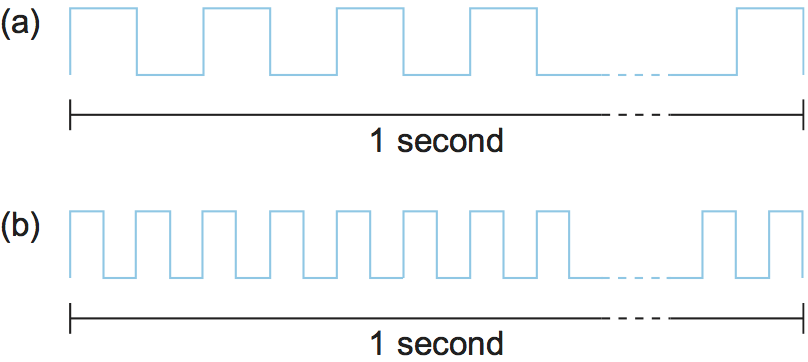
Figure 16. Bits transmitted at a particular bandwidth can be regarded as having some width: (a) bits transmitted at 1 Mbps (each bit is 1 microsecond wide); (b) bits transmitted at 2 Mbps (each bit is 0.5 microseconds wide).
The second performance metric, latency, corresponds to how long it takes a message to travel from one end of a network to the other. (As with bandwidth, we could be focused on the latency of a single link or an end-to-end channel.) Latency is measured strictly in terms of time. For example, a transcontinental network might have a latency of 24 milliseconds (ms); that is, it takes a message 24 ms to travel from one coast of North America to the other. There are many situations in which it is more important to know how long it takes to send a message from one end of a network to the other and back, rather than the one-way latency. We call this the round-trip time (RTT) of the network.
We often think of latency as having three components. First, there is the speed-of-light propagation delay. This delay occurs because nothing, including a bit on a wire, can travel faster than the speed of light. If you know the distance between two points, you can calculate the speed-of-light latency, although you have to be careful because light travels across different media at different speeds: It travels at 3.0 × 10⁸ m/s in a vacuum, 2.3 × 10⁸ m/s in a copper cable, and 2.0 × 10⁸ m/s in an optical fiber. Second, there is the amount of time it takes to transmit a unit of data. This is a function of the network bandwidth and the size of the packet in which the data is carried. Third, there may be queuing delays inside the network, since packet switches generally need to store packets for some time before forwarding them on an outbound link. So, we could define the total latency as
Latency = Propagation + Transmit + Queue
Propagation =  Distance/SpeedOfLight
Transmit = Size/Bandwidth
where Distance is the length of the wire over which the data will
travel, SpeedOfLight is the effective speed of light over that wire,
Size is the size of the packet, and Bandwidth is the bandwidth
at which the packet is transmitted. Note that if the message contains
only one bit and we are talking about a single link (as opposed to a
whole network), then the Transmit and Queue terms are not
relevant, and latency corresponds to the propagation delay only.
Bandwidth and latency combine to define the performance characteristics
of a given link or channel. Their relative importance, however, depends
on the application. For some applications, latency dominates bandwidth.
For example, a client that sends a 1-byte message to a server and
receives a 1-byte message in return is latency bound. Assuming that no
serious computation is involved in preparing the response, the
application will perform much differently on a transcontinental channel
with a 100-ms RTT than it will on an across-the-room channel with a
1-ms RTT. Whether the channel is 1 Mbps or 100 Mbps is relatively
insignificant, however, since the former implies that the time to
transmit a byte (Transmit) is 8 μs and the latter implies
Transmit = 0.08 μs.
In contrast, consider a digital library program that is being asked to fetch a 25-megabyte (MB) image—the more bandwidth that is available, the faster it will be able to return the image to the user. Here, the bandwidth of the channel dominates performance. To see this, suppose that the channel has a bandwidth of 10 Mbps. It will take 20 seconds to transmit the image (25 × 106 × 8-bits / (10 × 106 Mbps = 20 seconds), making it relatively unimportant if the image is on the other side of a 1-ms channel or a 100-ms channel; the difference between a 20.001-second response time and a 20.1-second response time is negligible.
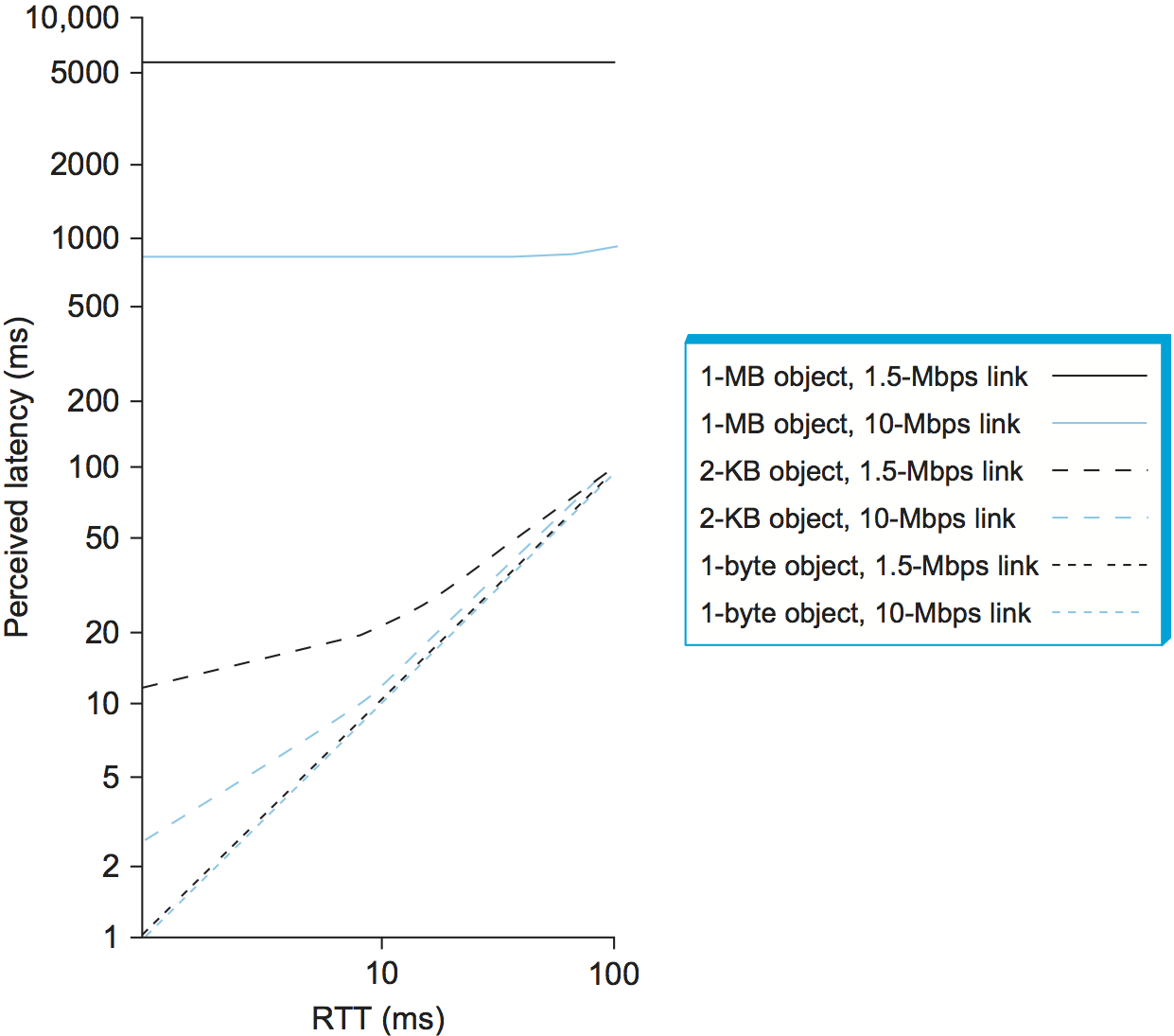
Figure 17. Perceived latency (response time) versus round-trip time for various object sizes and link speeds.
Figure 17 gives you a sense of how latency or bandwidth can dominate performance in different circumstances. The graph shows how long it takes to move objects of various sizes (1 byte, 2 KB, 1 MB) across networks with RTTs ranging from 1 to 100 ms and link speeds of either 1.5 or 10 Mbps. We use logarithmic scales to show relative performance. For a 1-byte object (say, a keystroke), latency remains almost exactly equal to the RTT, so that you cannot distinguish between a 1.5-Mbps network and a 10-Mbps network. For a 2-KB object (say, an email message), the link speed makes quite a difference on a 1-ms RTT network but a negligible difference on a 100-ms RTT network. And for a 1-MB object (say, a digital image), the RTT makes no difference—it is the link speed that dominates performance across the full range of RTT.
Note that throughout this book we use the terms latency and delay in a generic way to denote how long it takes to perform a particular function, such as delivering a message or moving an object. When we are referring to the specific amount of time it takes a signal to propagate from one end of a link to another, we use the term propagation delay. Also, we make it clear in the context of the discussion whether we are referring to the one-way latency or the round-trip time.
As an aside, computers are becoming so fast that when we connect them to networks, it is sometimes useful to think, at least figuratively, in terms of instructions per mile. Consider what happens when a computer that is able to execute 100 billion instructions per second sends a message out on a channel with a 100-ms RTT. (To make the math easier, assume that the message covers a distance of 5000 miles.) If that computer sits idle the full 100 ms waiting for a reply message, then it has forfeited the ability to execute 10 billion instructions, or 2 million instructions per mile. It had better have been worth going over the network to justify this waste.
1.5.2 Delay × Bandwidth Product
It is also useful to talk about the product of these two metrics, often called the delay × bandwidth product. Intuitively, if we think of a channel between a pair of processes as a hollow pipe (see Figure 18), where the latency corresponds to the length of the pipe and the bandwidth gives the diameter of the pipe, then the delay × bandwidth product gives the volume of the pipe—the maximum number of bits that could be in transit through the pipe at any given instant. Said another way, if latency (measured in time) corresponds to the length of the pipe, then given the width of each bit (also measured in time) you can calculate how many bits fit in the pipe. For example, a transcontinental channel with a one-way latency of 50 ms and a bandwidth of 45 Mbps is able to hold
50 × 10-3 × 45 × 106 bits/sec = 2.25 × 106 bits
or approximately 280 KB of data. In other words, this example channel (pipe) holds as many bytes as the memory of a personal computer from the early 1980s could hold.
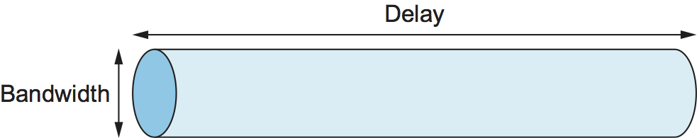
Figure 18. Network as a pipe.
The delay × bandwidth product is important to know when constructing high-performance networks because it corresponds to how many bits the sender must transmit before the first bit arrives at the receiver. If the sender is expecting the receiver to somehow signal that bits are starting to arrive, and it takes another channel latency for this signal to propagate back to the sender, then the sender can send up one RTT × bandwidth worth of data before hearing from the receiver that all is well. The bits in the pipe are said to be “in flight,” which means that if the receiver tells the sender to stop transmitting it might receive up to one RTT × bandwidth’s worth of data before the sender manages to respond. In our example above, that amount corresponds to 5.5 × 106 bits (671 KB) of data. On the other hand, if the sender does not fill the pipe—i.e., does not send a whole RTT × bandwidth product’s worth of data before it stops to wait for a signal—the sender will not fully utilize the network.
Note that most of the time we are interested in the RTT scenario, which we simply refer to as the delay × bandwidth product, without explicitly saying that “delay” is the RTT (i.e., multiply the one-way delay by two). Usually, whether the “delay” in delay × bandwidth means one-way latency or RTT is made clear by the context. Table 1 shows some examples of RTT × bandwidth products for some typical network links.
Link Type |
Bandwidth |
One-Way Distance |
RTT |
RTT x Bandwidth |
|---|---|---|---|---|
Wireless LAN |
54 Mbps |
50 m |
0.33 μs |
18 bits |
Satellite |
1 Gbps |
35,000 km |
230 ms |
230 Mb |
Cross-country fiber |
10 Gbps |
4,000 km |
40 ms |
400 Mb |
1.5.3 High-Speed Networks
The seeming continual increase in bandwidth causes network designers to start thinking about what happens in the limit or, stated another way, what is the impact on network design of having infinite bandwidth available.
Although high-speed networks bring a dramatic change in the bandwidth available to applications, in many respects their impact on how we think about networking comes in what does not change as bandwidth increases: the speed of light. To quote Scotty from Star Trek, “Ye cannae change the laws of physics.” In other words, “high speed” does not mean that latency improves at the same rate as bandwidth; the transcontinental RTT of a 1-Gbps link is the same 100 ms as it is for a 1-Mbps link.
To appreciate the significance of ever-increasing bandwidth in the face of fixed latency, consider what is required to transmit a 1-MB file over a 1-Mbps network versus over a 1-Gbps network, both of which have an RTT of 100 ms. In the case of the 1-Mbps network, it takes 80 round-trip times to transmit the file; during each RTT, 1.25% of the file is sent. In contrast, the same 1-MB file doesn’t even come close to filling 1 RTT’s worth of the 1-Gbps link, which has a delay × bandwidth product of 12.5 MB.
Figure 19 illustrates the difference between the two networks. In effect, the 1-MB file looks like a stream of data that needs to be transmitted across a 1-Mbps network, while it looks like a single packet on a 1-Gbps network. To help drive this point home, consider that a 1-MB file is to a 1-Gbps network what a 1-KB packet is to a 1-Mbps network.
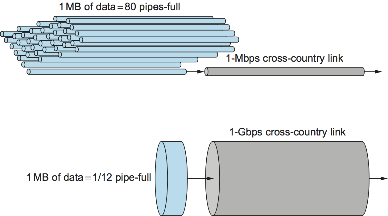
Figure 19. Relationship between bandwidth and latency. A 1-MB file would fill the 1-Mbps link 80 times but only fill 1/12th of a 1-Gbps link.
Another way to think about the situation is that more data can be transmitted during each RTT on a high-speed network, so much so that a single RTT becomes a significant amount of time. Thus, while you wouldn’t think twice about the difference between a file transfer taking 101 RTTs rather than 100 RTTs (a relative difference of only 1%), suddenly the difference between 1 RTT and 2 RTTs is significant—a 100% increase. In other words, latency, rather than throughput, starts to dominate our thinking about network design.
Perhaps the best way to understand the relationship between throughput and latency is to return to basics. The effective end-to-end throughput that can be achieved over a network is given by the simple relationship
Throughput = TransferSize / TransferTime
where TransferTime includes not only the elements of one-way identified earlier in this section, but also any additional time spent requesting or setting up the transfer. Generally, we represent this relationship as
TransferTime = RTT + 1/Bandwidth x TransferSize
We use in this calculation to account for a request message being sent across the network and the data being sent back. For example, consider a situation where a user wants to fetch a 1-MB file across a 1-Gbps with a round-trip time of 100 ms. This includes both the transmit time for 1 MB (1 / 1 Gbps × 1 MB = 8 ms) and the 100-ms RTT, for a total transfer time of 108 ms. This means that the effective throughput will be
1 MB / 108 ms = 74.1 Mbps
not 1 Gbps. Clearly, transferring a larger amount of data will help improve the effective throughput, where in the limit an infinitely large transfer size will cause the effective throughput to approach the network bandwidth. On the other hand, having to endure more than 1 RTT—for example, to retransmit missing packets—will hurt the effective throughput for any transfer of finite size and will be most noticeable for small transfers.
1.5.4 Application Requirements
The discussion in this section has taken a network-centric view of performance; that is, we have talked in terms of what a given link or channel will support. The unstated assumption has been that application programs have simple needs—they want as much bandwidth as the network can provide. This is certainly true of the aforementioned digital library program that is retrieving a 250-MB image; the more bandwidth that is available, the faster the program will be able to return the image to the user.
However, some applications are able to state an upper limit on how much bandwidth they need. Video applications are a prime example. Suppose one wants to stream a video that is one quarter the size of a standard TV screen; that is, it has a resolution of 352 by 240 pixels. If each pixel is represented by 24 bits of information, as would be the case for 24-bit color, then the size of each frame would be (352 × 240 × 24) / 8 = 247.5 KB If the application needs to support a frame rate of 30 frames per second, then it might request a throughput rate of 75 Mbps. The ability of the network to provide more bandwidth is of no interest to such an application because it has only so much data to transmit in a given period of time.
Unfortunately, the situation is not as simple as this example suggests. Because the difference between any two adjacent frames in a video stream is often small, it is possible to compress the video by transmitting only the differences between adjacent frames. Each frame can also be compressed because not all the detail in a picture is readily perceived by a human eye. The compressed video does not flow at a constant rate, but varies with time according to factors such as the amount of action and detail in the picture and the compression algorithm being used. Therefore, it is possible to say what the average bandwidth requirement will be, but the instantaneous rate may be more or less.
The key issue is the time interval over which the average is computed. Suppose that this example video application can be compressed down to the point that it needs only 2 Mbps, on average. If it transmits 1 megabit in a 1-second interval and 3 megabits in the following 1-second interval, then over the 2-second interval it is transmitting at an average rate of 2 Mbps; however, this will be of little consolation to a channel that was engineered to support no more than 2 megabits in any one second. Clearly, just knowing the average bandwidth needs of an application will not always suffice.
Generally, however, it is possible to put an upper bound on how large a burst an application like this is likely to transmit. A burst might be described by some peak rate that is maintained for some period of time. Alternatively, it could be described as the number of bytes that can be sent at the peak rate before reverting to the average rate or some lower rate. If this peak rate is higher than the available channel capacity, then the excess data will have to be buffered somewhere, to be transmitted later. Knowing how big of a burst might be sent allows the network designer to allocate sufficient buffer capacity to hold the burst.
Analogous to the way an application’s bandwidth needs can be something other than “all it can get,” an application’s delay requirements may be more complex than simply “as little delay as possible.” In the case of delay, it sometimes doesn’t matter so much whether the one-way latency of the network is 100 ms or 500 ms as how much the latency varies from packet to packet. The variation in latency is called jitter.
Consider the situation in which the source sends a packet once every 33 ms, as would be the case for a video application transmitting frames 30 times a second. If the packets arrive at the destination spaced out exactly 33 ms apart, then we can deduce that the delay experienced by each packet in the network was exactly the same. If the spacing between when packets arrive at the destination—sometimes called the inter-packet gap—is variable, however, then the delay experienced by the sequence of packets must have also been variable, and the network is said to have introduced jitter into the packet stream, as shown in Figure 20. Such variation is generally not introduced in a single physical link, but it can happen when packets experience different queuing delays in a multihop packet-switched network. This queuing delay corresponds to the component of latency defined earlier in this section, which varies with time.
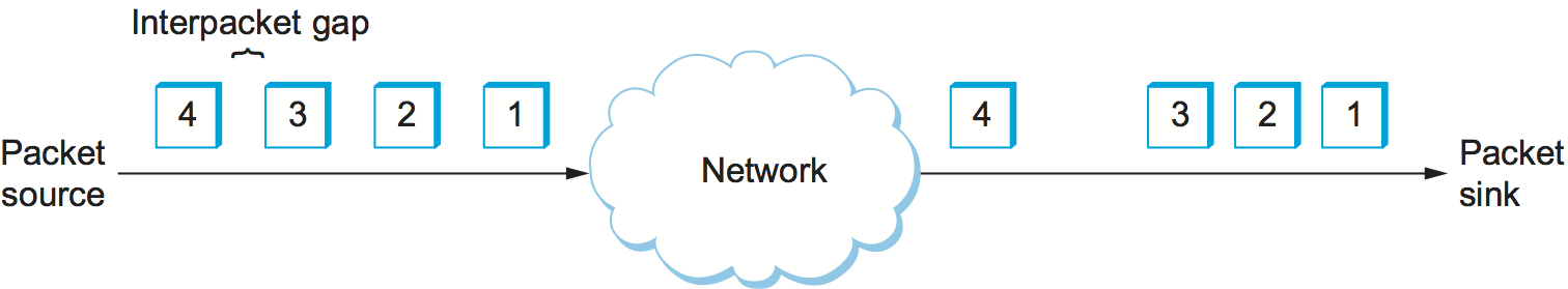
Figure 20. Network-induced jitter.
To understand the relevance of jitter, suppose that the packets being transmitted over the network contain video frames, and in order to display these frames on the screen the receiver needs to receive a new one every 33 ms. If a frame arrives early, then it can simply be saved by the receiver until it is time to display it. Unfortunately, if a frame arrives late, then the receiver will not have the frame it needs in time to update the screen, and the video quality will suffer; it will not be smooth. Note that it is not necessary to eliminate jitter, only to know how bad it is. The reason for this is that if the receiver knows the upper and lower bounds on the latency that a packet can experience, it can delay the time at which it starts playing back the video (i.e., displays the first frame) long enough to ensure that in the future it will always have a frame to display when it needs it. The receiver delays the frame, effectively smoothing out the jitter, by storing it in a buffer.