3.1 Switching Basics
In the simplest terms, a switch is a mechanism that allows us to interconnect links to form a larger network. A switch is a multi-input, multi-output device that transfers packets from an input to one or more outputs. Thus, a switch adds the star topology (see Figure 56) to the set of possible network structures. A star topology has several attractive properties:
Even though a switch has a fixed number of inputs and outputs, which limits the number of hosts that can be connected to a single switch, large networks can be built by interconnecting a number of switches.
We can connect switches to each other and to hosts using point-to-point links, which typically means that we can build networks of large geographic scope.
Adding a new host to the network by connecting it to a switch does not necessarily reduce the performance of the network for other hosts already connected.
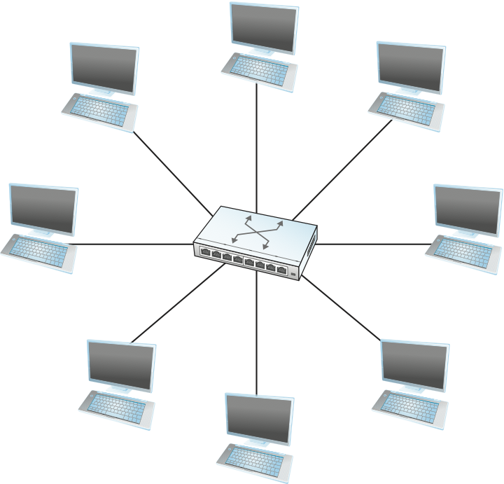
Figure 56. A switch provides a star topology.
This last claim cannot be made for the shared-media networks discussed in the last chapter. For example, it is impossible for two hosts on the same 10-Mbps Ethernet segment to transmit continuously at 10 Mbps because they share the same transmission medium. Every host on a switched network has its own link to the switch, so it may be entirely possible for many hosts to transmit at the full link speed (bandwidth), provided that the switch is designed with enough aggregate capacity. Providing high aggregate throughput is one of the design goals for a switch; we return to this topic later. In general, switched networks are considered more scalable (i.e., more capable of growing to large numbers of nodes) than shared-media networks because of this ability to support many hosts at full speed.
A switch is connected to a set of links and, for each of these links, runs the appropriate data link protocol to communicate with the node at the other end of the link. A switch’s primary job is to receive incoming packets on one of its links and to transmit them on some other link. This function is sometimes referred to as either switching or forwarding, and in terms of the Open Systems Interconnection (OSI) architecture, it is considered a function of the network layer. (This is a case where OSI layering isn’t a perfect reflection of the real world, as we’ll see later.)
The question, then, is how does the switch decide which output link to place each packet on? The general answer is that it looks at the header of the packet for an identifier that it uses to make the decision. The details of how it uses this identifier vary, but there are two common approaches. The first is the datagram or connectionless approach. The second is the virtual circuit or connection-oriented approach. A third approach, source routing, is less common than these other two, but it does have some useful applications.
One thing that is common to all networks is that we need to have a way to identify the end nodes. Such identifiers are usually called addresses. We have already seen examples of addresses, such as the 48-bit address used for Ethernet. The only requirement for Ethernet addresses is that no two nodes on a network have the same address. This is accomplished by making sure that all Ethernet cards are assigned a globally unique identifier. For the following discussion, we assume that each host has a globally unique address. Later on, we consider other useful properties that an address might have, but global uniqueness is adequate to get us started.
Another assumption that we need to make is that there is some way to identify the input and output ports of each switch. There are at least two sensible ways to identify ports: One is to number each port, and the other is to identify the port by the name of the node (switch or host) to which it leads. For now, we use numbering of the ports.
3.1.1 Datagrams
The idea behind datagrams is incredibly simple: You just include in every packet enough information to enable any switch to decide how to get it to its destination. That is, every packet contains the complete destination address. Consider the example network illustrated in Figure 57, in which the hosts have addresses A, B, C, and so on. To decide how to forward a packet, a switch consults a forwarding table (sometimes called a routing table), an example of which is depicted in Table 5. This particular table shows the forwarding information that switch 2 needs to forward datagrams in the example network. It is pretty easy to figure out such a table when you have a complete map of a simple network like that depicted here; we could imagine a network operator configuring the tables statically. It is a lot harder to create the forwarding tables in large, complex networks with dynamically changing topologies and multiple paths between destinations. That harder problem is known as routing and is the topic of a later section. We can think of routing as a process that takes place in the background so that, when a data packet turns up, we will have the right information in the forwarding table to be able to forward, or switch, the packet.
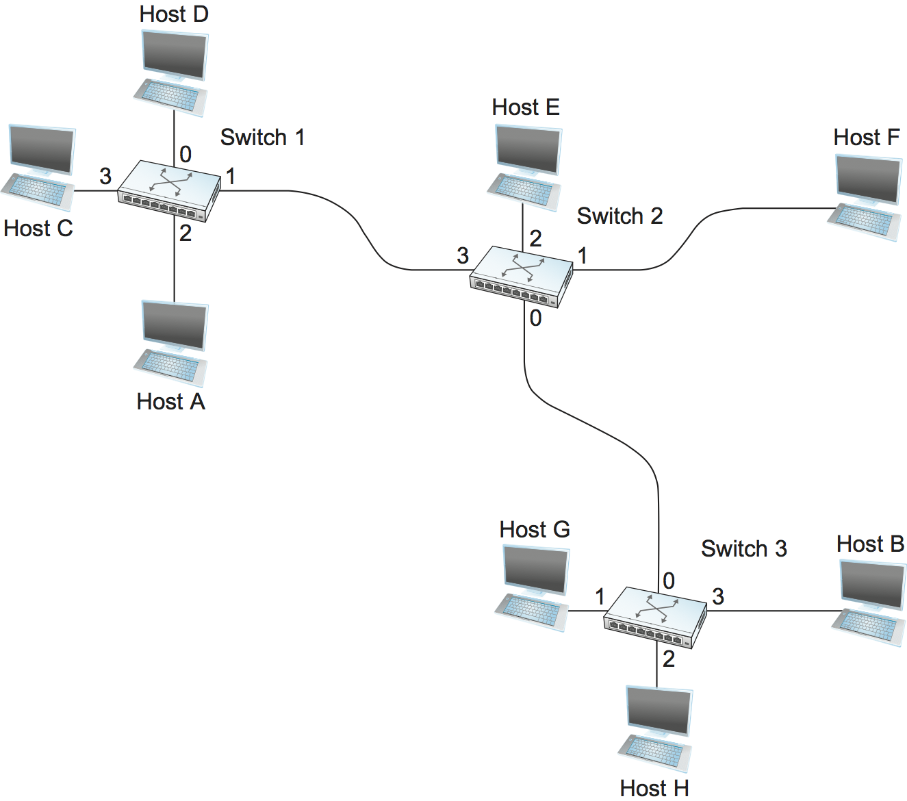
Figure 57. Datagram forwarding: an example network.
Destination |
Port |
|---|---|
A |
3 |
B |
0 |
C |
3 |
D |
3 |
E |
2 |
F |
1 |
G |
0 |
H |
0 |
Datagram networks have the following characteristics:
A host can send a packet anywhere at any time, since any packet that turns up at a switch can be immediately forwarded (assuming a correctly populated forwarding table). For this reason, datagram networks are often called connectionless; this contrasts with the connection-oriented networks described below, in which some connection state needs to be established before the first data packet is sent.
When a host sends a packet, it has no way of knowing if the network is capable of delivering it or if the destination host is even up and running.
Each packet is forwarded independently of previous packets that might have been sent to the same destination. Thus, two successive packets from host A to host B may follow completely different paths (perhaps because of a change in the forwarding table at some switch in the network).
A switch or link failure might not have any serious effect on communication if it is possible to find an alternate route around the failure and to update the forwarding table accordingly.
This last fact is particularly important to the history of datagram networks. One of the important design goals of the Internet is robustness to failures, and history has shown it to be quite effective at meeting this goal. Since datagram-based networks are the dominant technology discussed in this book, we postpone illustrative examples for the following sections, and move on to the two main alternatives.
3.1.2 Virtual Circuit Switching
A second technique for packet switching uses the concept of a virtual circuit (VC). This approach, which is also referred to as a connection-oriented model, requires setting up a virtual connection from the source host to the destination host before any data is sent. To understand how this works, consider Figure 58, where host A again wants to send packets to host B. We can think of this as a two-stage process. The first stage is “connection setup.” The second is data transfer. We consider each in turn.
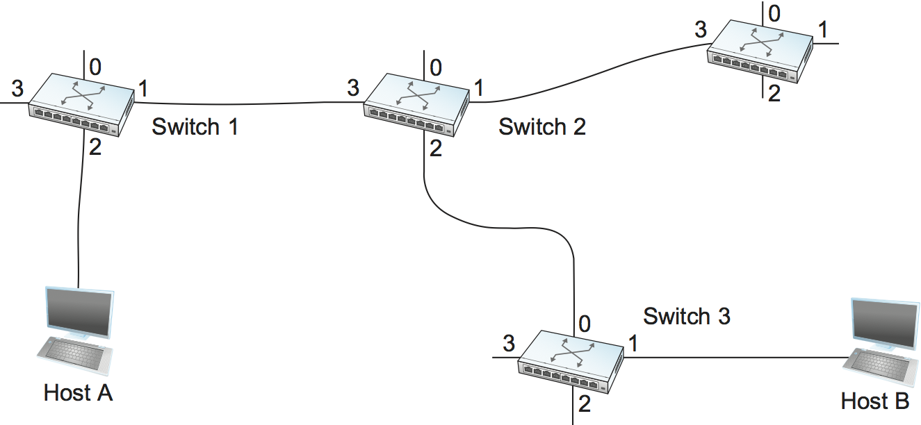
Figure 58. An example of a virtual circuit network.
In the connection setup phase, it is necessary to establish a “connection state” in each of the switches between the source and destination hosts. The connection state for a single connection consists of an entry in a “VC table” in each switch through which the connection passes. One entry in the VC table on a single switch contains:
A virtual circuit identifier (VCI) that uniquely identifies the connection at this switch and which will be carried inside the header of the packets that belong to this connection
An incoming interface on which packets for this VC arrive at the switch
An outgoing interface in which packets for this VC leave the switch
A potentially different VCI that will be used for outgoing packets
The semantics of one such entry is as follows: If a packet arrives on the designated incoming interface and that packet contains the designated VCI value in its header, then that packet should be sent out the specified outgoing interface with the specified outgoing VCI value having been first placed in its header.
Note that the combination of the VCI of packets as they are received at the switch and the interface on which they are received uniquely identifies the virtual connection. There may of course be many virtual connections established in the switch at one time. Also, we observe that the incoming and outgoing VCI values are generally not the same. Thus, the VCI is not a globally significant identifier for the connection; rather, it has significance only on a given link (i.e., it has link-local scope).
Whenever a new connection is created, we need to assign a new VCI for that connection on each link that the connection will traverse. We also need to ensure that the chosen VCI on a given link is not currently in use on that link by some existing connection.
There are two broad approaches to establishing connection state. One is to have a network administrator configure the state, in which case the virtual circuit is “permanent.” Of course, it can also be deleted by the administrator, so a permanent virtual circuit (PVC) might best be thought of as a long-lived or administratively configured VC. Alternatively, a host can send messages into the network to cause the state to be established. This is referred to as signalling, and the resulting virtual circuits are said to be switched. The salient characteristic of a switched virtual circuit (SVC) is that a host may set up and delete such a VC dynamically without the involvement of a network administrator. Note that an SVC should more accurately be called a signalled VC, since it is the use of signalling (not switching) that distinguishes an SVC from a PVC.
Let’s assume that a network administrator wants to manually create a new virtual connection from host A to host B. First, the administrator needs to identify a path through the network from A to B. In the example network of Figure 58, there is only one such path, but in general, this may not be the case. The administrator then picks a VCI value that is currently unused on each link for the connection. For the purposes of our example, let’s suppose that the VCI value 5 is chosen for the link from host A to switch 1, and that 11 is chosen for the link from switch 1 to switch 2. In that case, switch 1 needs to have an entry in its VC table configured as shown in Table 6.
Incoming Interface |
Incoming VCI |
Outgoing Interface |
Outgoing VCI |
|---|---|---|---|
2 |
5 |
1 |
11 |
Similarly, suppose that the VCI of 7 is chosen to identify this connection on the link from switch 2 to switch 3 and that a VCI of 4 is chosen for the link from switch 3 to host B. In that case, switches 2 and 3 need to be configured with VC table entries as shown in Table 7 and Table 8, respectively. Note that the “outgoing” VCI value at one switch is the “incoming” VCI value at the next switch.
Incoming Interface |
Incoming VCI |
Outgoing Interface |
Outgoing VCI |
|---|---|---|---|
3 |
11 |
2 |
7 |
Incoming Interface |
Incoming VCI |
Outgoing Interface |
Outgoing VCI |
|---|---|---|---|
0 |
7 |
1 |
4 |
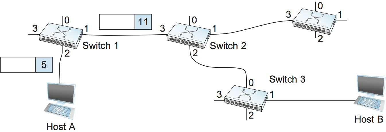
Figure 59. A packet is sent into a virtual circuit network.
Once the VC tables have been set up, the data transfer phase can proceed, as illustrated in Figure 59. For any packet that it wants to send to host B, A puts the VCI value of 5 in the header of the packet and sends it to switch 1. Switch 1 receives any such packet on interface 2, and it uses the combination of the interface and the VCI in the packet header to find the appropriate VC table entry. As shown in Table 6, the table entry in this case tells switch 1 to forward the packet out of interface 1 and to put the VCI value 11 in the header when the packet is sent. Thus, the packet will arrive at switch 2 on interface 3 bearing VCI 11. Switch 2 looks up interface 3 and VCI 11 in its VC table (as shown in Table 7) and sends the packet on to switch 3 after updating the VCI value in the packet header appropriately, as shown in Figure 60. This process continues until it arrives at host B with the VCI value of 4 in the packet. To host B, this identifies the packet as having come from host A.
In real networks of reasonable size, the burden of configuring VC tables correctly in a large number of switches would quickly become excessive using the above procedures. Thus, either a network management tool or some sort of signalling (or both) is almost always used, even when setting up “permanent” VCs. In the case of PVCs, signalling is initiated by the network administrator, while SVCs are usually set up using signalling by one of the hosts. We consider now how the same VC just described could be set up by signalling from the host.
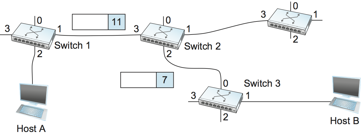
Figure 60. A packet makes its way through a virtual circuit network.
To start the signalling process, host A sends a setup message into the network—that is, to switch 1. The setup message contains, among other things, the complete destination address of host B. The setup message needs to get all the way to B to create the necessary connection state in every switch along the way. We can see that getting the setup message to B is a lot like getting a datagram to B, in that the switches have to know which output to send the setup message to so that it eventually reaches B. For now, let’s just assume that the switches know enough about the network topology to figure out how to do that, so that the setup message flows on to switches 2 and 3 before finally reaching host B.
When switch 1 receives the connection request, in addition to sending it on to switch 2, it creates a new entry in its virtual circuit table for this new connection. This entry is exactly the same as shown previously in Table 6. The main difference is that now the task of assigning an unused VCI value on the interface is performed by the switch for that port. In this example, the switch picks the value 5. The virtual circuit table now has the following information: “When packets arrive on port 2 with identifier 5, send them out on port 1.” Another issue is that, somehow, host A will need to learn that it should put the VCI value of 5 in packets that it wants to send to B; we will see how that happens below.
When switch 2 receives the setup message, it performs a similar process; in this example, it picks the value 11 as the incoming VCI value. Similarly, switch 3 picks 7 as the value for its incoming VCI. Each switch can pick any number it likes, as long as that number is not currently in use for some other connection on that port of that switch. As noted above, VCIs have link-local scope; that is, they have no global significance.
Finally, the setup message arrives as host B. Assuming that B is healthy and willing to accept a connection from host A, it too allocates an incoming VCI value, in this case 4. This VCI value can be used by B to identify all packets coming from host A.
Now, to complete the connection, everyone needs to be told what their downstream neighbor is using as the VCI for this connection. Host B sends an acknowledgment of the connection setup to switch 3 and includes in that message the VCI that it chose (4). Now switch 3 can complete the virtual circuit table entry for this connection, since it knows the outgoing value must be 4. Switch 3 sends the acknowledgment on to switch 2, specifying a VCI of 7. Switch 2 sends the message on to switch 1, specifying a VCI of 11. Finally, switch 1 passes the acknowledgment on to host A, telling it to use the VCI of 5 for this connection.
At this point, everyone knows all that is necessary to allow traffic to flow from host A to host B. Each switch has a complete virtual circuit table entry for the connection. Furthermore, host A has a firm acknowledgment that everything is in place all the way to host B. At this point, the connection table entries are in place in all three switches just as in the administratively configured example above, but the whole process happened automatically in response to the signalling message sent from A. The data transfer phase can now begin and is identical to that used in the PVC case.
When host A no longer wants to send data to host B, it tears down the connection by sending a teardown message to switch 1. The switch removes the relevant entry from its table and forwards the message on to the other switches in the path, which similarly delete the appropriate table entries. At this point, if host A were to send a packet with a VCI of 5 to switch 1, it would be dropped as if the connection had never existed.
There are several things to note about virtual circuit switching:
Since host A has to wait for the connection request to reach the far side of the network and return before it can send its first data packet, there is at least one round-trip time (RTT) of delay before data is sent.
While the connection request contains the full address for host B (which might be quite large, being a global identifier on the network), each data packet contains only a small identifier, which is only unique on one link. Thus, the per-packet overhead caused by the header is reduced relative to the datagram model. More importantly, the lookup is fast because the virtual circuit number can be treated as an index into a table rather than as a key that has to be looked up.
If a switch or a link in a connection fails, the connection is broken and a new one will need to be established. Also, the old one needs to be torn down to free up table storage space in the switches.
The issue of how a switch decides which link to forward the connection request on has been glossed over. In essence, this is the same problem as building up the forwarding table for datagram forwarding, which requires some sort of routing algorithm. Routing is described in a later section, and the algorithms described there are generally applicable to routing setup requests as well as datagrams.
One of the nice aspects of virtual circuits is that by the time the host gets the go-ahead to send data, it knows quite a lot about the network—for example, that there really is a route to the receiver and that the receiver is willing and able to receive data. It is also possible to allocate resources to the virtual circuit at the time it is established. For example, X.25 (an early and now largely obsolete virtual-circuit-based networking technology) employed the following three-part strategy:
Buffers are allocated to each virtual circuit when the circuit is initialized.
The sliding window protocol is run between each pair of nodes along the virtual circuit, and this protocol is augmented with flow control to keep the sending node from over-running the buffers allocated at the receiving node.
The circuit is rejected by a given node if not enough buffers are available at that node when the connection request message is processed.
In doing these three things, each node is ensured of having the buffers it needs to queue the packets that arrive on that circuit. This basic strategy is usually called hop-by-hop flow control.
By comparison, a datagram network has no connection establishment phase, and each switch processes each packet independently, making it less obvious how a datagram network would allocate resources in a meaningful way. Instead, each arriving packet competes with all other packets for buffer space. If there are no free buffers, the incoming packet must be discarded. We observe, however, that even in a datagram-based network a source host often sends a sequence of packets to the same destination host. It is possible for each switch to distinguish among the set of packets it currently has queued, based on the source/destination pair, and thus for the switch to ensure that the packets belonging to each source/destination pair are receiving a fair share of the switch’s buffers.
In the virtual circuit model, we could imagine providing each circuit with a different quality of service (QoS). In this setting, the term quality of service is usually taken to mean that the network gives the user some kind of performance-related guarantee, which in turn implies that switches set aside the resources they need to meet this guarantee. For example, the switches along a given virtual circuit might allocate a percentage of each outgoing link’s bandwidth to that circuit. As another example, a sequence of switches might ensure that packets belonging to a particular circuit not be delayed (queued) for more than a certain amount of time.
There have been a number of successful examples of virtual circuit technologies over the years, notably X.25, Frame Relay, and Asynchronous Transfer Mode (ATM). With the success of the Internet’s connectionless model, however, none of them enjoys great popularity today. One of the most common applications of virtual circuits for many years was the construction of virtual private networks (VPNs), a subject discussed in a later section. Even that application is now mostly supported using Internet-based technologies today.
Asynchronous Transfer Mode (ATM)
Asynchronous Transfer Mode (ATM) is probably the most well-known virtual circuit-based networking technology, although it is now well past its peak in terms of deployment. ATM became an important technology in the 1980s and early 1990s for a variety of reasons, not the least of which is that it was embraced by the telephone industry, which at that point in time was less active in computer networks (other than as a supplier of links from which other people built networks). ATM also happened to be in the right place at the right time, as a high-speed switching technology that appeared on the scene just when shared media like Ethernet and token rings were starting to look a bit too slow for many users of computer networks. In some ways ATM was a competing technology with Ethernet switching, and it was seen by many as a competitor to IP as well.
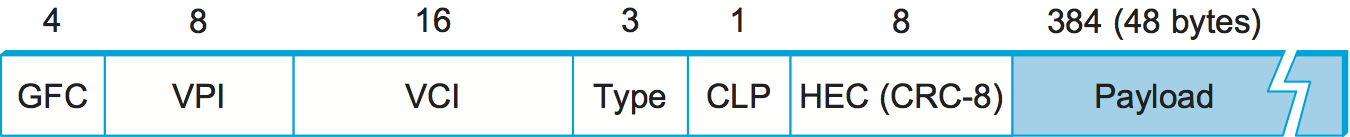
Figure 61. ATM cell format at the UNI.
The approach ATM takes has some interesting properties, which makes it worth examining a bit further. The picture of the ATM packet format—more commonly called an ATM cell—in Figure 61 will illustrate the main points. We’ll skip the generic flow control (GFC) bits, which never saw much use, and start with the 24 bits that are labelled VPI (virtual path identifier—8 bits) and VCI (virtual circuit identifier—16 bits). If you consider these bits together as a single 24-bit field, they correspond to the virtual circuit identifier introduced above. The reason for breaking the field into two parts was to allow for a level of hierarchy: All the circuits with the same VPI could, in some cases, be treated as a group (a virtual path) and could all be switched together looking only at the VPI, simplifying the work of a switch that could ignore all the VCI bits and reducing the size of the VC table considerably.
Skipping to the last header byte we find an 8-bit cyclic redundancy
check (CRC), known as the header error check (HEC). It uses CRC-8
and provides error detection and single-bit error correction capability
on the cell header only. Protecting the cell header is particularly
important because an error in the VCI will cause the cell to be
misdelivered.
Probably the most significant thing to notice about the ATM cell, and the reason it is called a cell and not a packet, is that it comes in only one size: 53 bytes. What was the reason for this? One big reason was to facilitate the implementation of hardware switches. When ATM was being created in the mid- and late 1980s, 10-Mbps Ethernet was the cutting-edge technology in terms of speed. To go much faster, most people thought in terms of hardware. Also, in the telephone world, people think big when they think of switches—telephone switches often serve tens of thousands of customers. Fixed-length packets turn out to be a very helpful thing if you want to build fast, highly scalable switches. There are two main reasons for this:
It is easier to build hardware to do simple jobs, and the job of processing packets is simpler when you already know how long each one will be.
If all packets are the same length, then you can have lots of switching elements all doing much the same thing in parallel, each of them taking the same time to do its job.
This second reason, the enabling of parallelism, greatly improves the scalability of switch designs. It would be overstating the case to say that fast parallel hardware switches can only be built using fixed-length cells. However, it is certainly true that cells ease the task of building such hardware and that there was a lot of knowledge available about how to build cell switches in hardware at the time the ATM standards were being defined. As it turns out, this same principle is still applied in many switches and routers today, even if they deal in variable length packets—they cut those packets into some sort of cell in order to forward them from input port to output port, but this is all internal to the switch.
There is another good argument in favor of small ATM cells, having to do with end-to-end latency. ATM was designed to carry both voice phone calls (the dominant use case at the time) and data. Because voice is low-bandwidth but has strict delay requirements, the last thing you want is for a small voice packet queued behind a large data packet at a switch. If you force all packets to be small (i.e., cell-sized), then large data packets can still be supported by reassembling a set of cells into a packet, and you get the benefit of being able to interleave the forwarding of voice cells and data cells at every switch along the path from source to destination. This idea of using small cells to improve end-to-end latency is alive and well today in cellular access networks.
Having decided to use small, fixed-length packets, the next question was what is the right length to fix them at? If you make them too short, then the amount of header information that needs to be carried around relative to the amount of data that fits in one cell gets larger, so the percentage of link bandwidth that is actually used to carry data goes down. Even more seriously, if you build a device that processes cells at some maximum number of cells per second, then as cells get shorter the total data rate drops in direct proportion to cell size. An example of such a device might be a network adaptor that reassembles cells into larger units before handing them up to the host. The performance of such a device depends directly on cell size. On the other hand, if you make the cells too big, then there is a problem of wasted bandwidth caused by the need to pad transmitted data to fill a complete cell. If the cell payload size is 48 bytes and you want to send 1 byte, you’ll need to send 47 bytes of padding. If this happens a lot, then the utilization of the link will be very low. The combination of relatively high header-to-payload ratio plus the frequency of sending partially filled cells did actually lead to some noticeable inefficiency in ATM networks that some detractors called the cell tax.
As it turns out, 48 bytes was picked for the ATM cell payload as a compromise. There were good arguments for both larger and smaller cells, and 48 made almost no one happy—a power of two would certainly have been better for computers to process.
3.1.3 Source Routing
A third approach to switching that uses neither virtual circuits nor conventional datagrams is known as source routing. The name derives from the fact that all the information about network topology that is required to switch a packet across the network is provided by the source host.
There are various ways to implement source routing. One would be to assign a number to each output of each switch and to place that number in the header of the packet. The switching function is then very simple: For each packet that arrives on an input, the switch would read the port number in the header and transmit the packet on that output. However, since there will in general be more than one switch in the path between the sending and the receiving host, the header for the packet needs to contain enough information to allow every switch in the path to determine which output the packet needs to be placed on. One way to do this would be to put an ordered list of switch ports in the header and to rotate the list so that the next switch in the path is always at the front of the list. Figure 62 illustrates this idea.
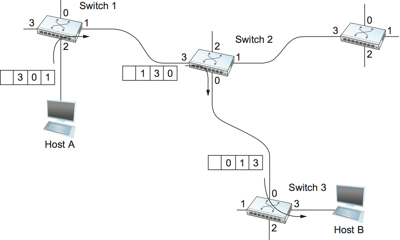
Figure 62. Source routing in a switched network (where the switch reads the rightmost number).
In this example, the packet needs to traverse three switches to get from host A to host B. At switch 1, it needs to exit on port 1, at the next switch it needs to exit at port 0, and at the third switch it needs to exit at port 3. Thus, the original header when the packet leaves host A contains the list of ports (3, 0, 1), where we assume that each switch reads the rightmost element of the list. To make sure that the next switch gets the appropriate information, each switch rotates the list after it has read its own entry. Thus, the packet header as it leaves switch 1 en route to switch 2 is now (1, 3, 0); switch 2 performs another rotation and sends out a packet with (0, 1, 3) in the header. Although not shown, switch 3 performs yet another rotation, restoring the header to what it was when host A sent it.
There are several things to note about this approach. First, it assumes that host A knows enough about the topology of the network to form a header that has all the right directions in it for every switch in the path. This is somewhat analogous to the problem of building the forwarding tables in a datagram network or figuring out where to send a setup packet in a virtual circuit network. In practice, however, it is the first switch at the ingress to the network (as opposed to the end host connected to that switch) that appends the source route.
Second, observe that we cannot predict how big the header needs to be, since it must be able to hold one word of information for every switch on the path. This implies that headers are probably of variable length with no upper bound, unless we can predict with absolute certainty the maximum number of switches through which a packet will ever need to pass.
Third, there are some variations on this approach. For example, rather
than rotate the header, each switch could just strip the first element
as it uses it. Rotation has an advantage over stripping, however: Host B
gets a copy of the complete header, which may help it figure out how to
get back to host A. Yet another alternative is to have the header carry
a pointer to the current “next port” entry, so that each switch just
updates the pointer rather than rotating the header; this may be more
efficient to implement. We show these three approaches in
Figure 63. In each case, the entry that
this switch needs to read is A, and the entry that the next switch
needs to read is B.
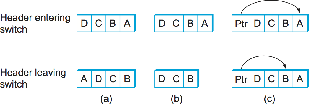
Figure 63. Three ways to handle headers for source routing: (a) rotation; (b) stripping; (c) pointer. The labels are read right to left.
Source routing can be used in both datagram networks and virtual circuit networks. For example, the Internet Protocol, which is a datagram protocol, includes a source route option that allows selected packets to be source routed, while the majority are switched as conventional datagrams. Source routing is also used in some virtual circuit networks as the means to get the initial setup request along the path from source to destination.
Source routes are sometimes categorized as strict or loose. In a strict source route, every node along the path must be specified, whereas a loose source route only specifies a set of nodes to be traversed, without saying exactly how to get from one node to the next. A loose source route can be thought of as a set of waypoints rather than a completely specified route. The loose option can be helpful to limit the amount of information that a source must obtain to create a source route. In any reasonably large network, it is likely to be hard for a host to get the complete path information it needs to construct correctly a strict source route to any destination. But both types of source routes do find application in certain scenarios, as we will see in later chapters.