4.2 IP Version 6

The motivation for defining a new version of IP is simple: to deal with exhaustion of the IP address space. CIDR helped considerably to contain the rate at which the Internet address space was being consumed and also helped to control the growth of routing table information needed in the Internet’s routers. However, these techniques are no longer adequate. In particular, it is virtually impossible to achieve 100% address utilization efficiency, so the address space was consumed well before the 4 billionth host was connected to the Internet. Even if we were able to use all 4 billion addresses, it is now clear that IP addresses need to be assigned to more than traditional computers, including smart phones, televisions, household appliances, and drones. With the clarity of 20/20 hindsight, a 32-bit address space is quite small.

4.2.1 Historical Perspective

The IETF began looking at the problem of expanding the IP address space in 1991, and several alternatives were proposed. Since the IP address is carried in the header of every IP packet, increasing the size of the address dictates a change in the packet header. This means a new version of the Internet Protocol and, as a consequence, a need for new software for every host and router in the Internet. This is clearly not a trivial matter—it is a major change that needs to be thought about very carefully.

The effort to define a new version of IP was originally known as IP Next Generation, or IPng. As the work progressed, an official IP version number was assigned, so IPng became IPv6. Note that the version of IP discussed so far in this chapter is version 4 (IPv4). The apparent discontinuity in numbering is the result of version number 5 being used for an experimental protocol many years ago.

The significance of changing to a new version of IP caused a snowball effect. The general feeling among network designers was that if you are going to make a change of this magnitude you might as well fix as many other things in IP as possible at the same time. Consequently, the IETF solicited white papers from anyone who cared to write one, asking for input on the features that might be desired in a new version of IP. In addition to the need to accommodate scalable routing and addressing, some of the other wish list items for IPng included:

• Support for real-time services

• Security support

• Autoconfiguration (i.e., the ability of hosts to automatically configure themselves with such information as their own IP address and domain name)

• Enhanced routing functionality, including support for mobile hosts

It is interesting to note that, while many of these features were absent from IPv4 at the time IPv6 was being designed, support for all of them has made its way into IPv4 in recent years, often using similar techniques in both protocols. It can be argued that the freedom to think of IPv6 as a clean slate facilitated the design of new capabilities for IP that were then retrofitted into IPv4.

In addition to the wish list, one absolutely non-negotiable feature for IPv6 was that there must be a transition plan to move from the current version of IP (version 4) to the new version. With the Internet being so large and having no centralized control, it would be completely impossible to have a “flag day” on which everyone shut down their hosts and routers and installed a new version of IP. The architects expected a long transition period in which some hosts and routers would run IPv4 only, some will run IPv4 and IPv6, and some will run IPv6 only. It is doubtful they anticipated that transition period would be approaching its 30th anniversary.

4.2.2 Addresses and Routing

First and foremost, IPv6 provides a 128-bit address space, as opposed to the 32 bits of version 4. Thus, while version 4 can potentially address 4 billion nodes if address assignment efficiency reaches 100%, IPv6 can address 3.4 × 10³⁸ nodes, again assuming 100% efficiency. As we have seen, though, 100% efficiency in address assignment is not likely. Some analysis of other addressing schemes, such as those of the French and U.S. telephone networks, as well as that of IPv4, have turned up some empirical numbers for address assignment efficiency. Based on the most pessimistic estimates of efficiency drawn from this study, the IPv6 address space is predicted to provide over 1500 addresses per square foot of the Earth’s surface, which certainly seems like it should serve us well even when toasters on Venus have IP addresses.

Address Space Allocation

Drawing on the effectiveness of CIDR in IPv4, IPv6 addresses are also classless, but the address space is still subdivided in various ways based on the leading bits. Rather than specifying different address classes, the leading bits specify different uses of the IPv6 address. The current assignment of prefixes is listed in Table 21.

Table 21. Address Prefix Assignments for IPv6.

Prefix	Use
00…0 (128 bits)	Unspecified
00…1 (128 bits)	Loopback
1111 1111	Multicast addresses
1111 1110 10	Link-local unicast
Everything else	Global Unicast

This allocation of the address space warrants a little discussion. First, the entire functionality of IPv4’s three main address classes (A, B, and C) is contained inside the “everything else” range. Global Unicast Addresses, as we will see shortly, are a lot like classless IPv4 addresses, only much longer. These are the main ones of interest at this point, with over 99% of the total IPv6 address space available to this important form of address. (At the time of writing, IPv6 unicast addresses are being allocated from the block that begins 001, with the remaining address space—about 87%—being reserved for future use.)

The multicast address space is (obviously) for multicast, thereby serving the same role as class D addresses in IPv4. Note that multicast addresses are easy to distinguish—they start with a byte of all 1s. We will see how these addresses are used in a later section.

The idea behind link-local use addresses is to enable a host to construct an address that will work on the network to which it is connected without being concerned about the global uniqueness of the address. This may be useful for autoconfiguration, as we will see below. Similarly, the site-local use addresses are intended to allow valid addresses to be constructed on a site (e.g., a private corporate network) that is not connected to the larger Internet; again, global uniqueness need not be an issue.

Within the global unicast address space are some important special types of addresses. A node may be assigned an IPv4-compatible IPv6 address by zero-extending a 32-bit IPv4 address to 128 bits. A node that is only capable of understanding IPv4 can be assigned an IPv4-mapped IPv6 address by prefixing the 32-bit IPv4 address with 2 bytes of all 1s and then zero-extending the result to 128 bits. These two special address types have uses in the IPv4-to-IPv6 transition (see the sidebar on this topic).

Address Notation

Just as with IPv4, there is some special notation for writing down IPv6 addresses. The standard representation is x:x:x:x:x:x:x:x, where each x is a hexadecimal representation of a 16-bit piece of the address. An example would be

47CD:1234:4422:AC02:0022:1234:A456:0124

Any IPv6 address can be written using this notation. Since there are a few special types of IPv6 addresses, there are some special notations that may be helpful in certain circumstances. For example, an address with a large number of contiguous 0s can be written more compactly by omitting all the 0 fields. Thus,

47CD:0000:0000:0000:0000:0000:A456:0124

could be written

47CD::A456:0124

Clearly, this form of shorthand can only be used for one set of contiguous 0s in an address to avoid ambiguity.

The two types of IPv6 addresses that contain an embedded IPv4 address have their own special notation that makes extraction of the IPv4 address easier. For example, the IPv4-mapped IPv6 address of a host whose IPv4 address was 128.96.33.81 could be written as

::FFFF:128.96.33.81

That is, the last 32 bits are written in IPv4 notation, rather than as a pair of hexadecimal numbers separated by a colon. Note that the double colon at the front indicates the leading 0s.

Global Unicast Addresses

By far the most important sort of addressing that IPv6 must provide is plain old unicast addressing. It must do this in a way that supports the rapid rate of addition of new hosts to the Internet and that allows routing to be done in a scalable way as the number of physical networks in the Internet grows. Thus, at the heart of IPv6 is the unicast address allocation plan that determines how unicast addresses will be assigned to service providers, autonomous systems, networks, hosts, and routers.

In fact, the address allocation plan that is proposed for IPv6 unicast addresses is extremely similar to that being deployed with CIDR in IPv4. To understand how it works and how it provides scalability, it is helpful to define some new terms. We may think of a nontransit AS (i.e., a stub or multihomed AS) as a subscriber, and we may think of a transit AS as a provider. Furthermore, we may subdivide providers into direct and indirect. The former are directly connected to subscribers. The latter primarily connect other providers, are not connected directly to subscribers, and are often known as backbone networks.

With this set of definitions, we can see that the Internet is not just an arbitrarily interconnected set of autonomous systems; it has some intrinsic hierarchy. The difficulty lies in making use of this hierarchy without inventing mechanisms that fail when the hierarchy is not strictly observed, as happened with EGP. For example, the distinction between direct and indirect providers becomes blurred when a subscriber connects to a backbone or when a direct provider starts connecting to many other providers.

As with CIDR, the goal of the IPv6 address allocation plan is to provide aggregation of routing information to reduce the burden on intradomain routers. Again, the key idea is to use an address prefix—a set of contiguous bits at the most significant end of the address—to aggregate reachability information to a large number of networks and even to a large number of autonomous systems. The main way to achieve this is to assign an address prefix to a direct provider and then for that direct provider to assign longer prefixes that begin with that prefix to its subscribers. Thus, a provider can advertise a single prefix for all of its subscribers.

Of course, the drawback is that if a site decides to change providers, it will need to obtain a new address prefix and renumber all the nodes in the site. This could be a colossal undertaking, enough to dissuade most people from ever changing providers. For this reason, there is ongoing research on other addressing schemes, such as geographic addressing, in which a site’s address is a function of its location rather than the provider to which it attaches. At present, however, provider-based addressing is necessary to make routing work efficiently.

Note that while IPv6 address assignment is essentially equivalent to the way address assignment has happened in IPv4 since the introduction of CIDR, IPv6 has the significant advantage of not having a large installed base of assigned addresses to fit into its plans.

One question is whether it makes sense for hierarchical aggregation to take place at other levels in the hierarchy. For example, should all providers obtain their address prefixes from within a prefix allocated to the backbone to which they connect? Given that most providers connect to multiple backbones, this probably doesn’t make sense. Also, since the number of providers is much smaller than the number of sites, the benefits of aggregating at this level are much fewer.

One place where aggregation may make sense is at the national or continental level. Continental boundaries form natural divisions in the Internet topology. If all addresses in Europe, for example, had a common prefix, then a great deal of aggregation could be done, and most routers in other continents would only need one routing table entry for all networks with the Europe prefix. Providers in Europe would all select their prefixes such that they began with the European prefix. Using this scheme, an IPv6 address might look like Figure 107. The RegistryID might be an identifier assigned to a European address registry, with different IDs assigned to other continents or countries. Note that prefixes would be of different lengths under this scenario. For example, a provider with few customers could have a longer prefix (and thus less total address space available) than one with many customers.

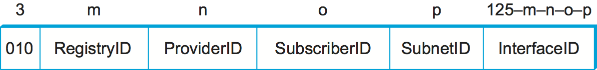
Figure 107. An IPv6 provider-based unicast address.

One tricky situation could occur when a subscriber is connected to more than one provider. Which prefix should the subscriber use for his or her site? There is no perfect solution to the problem. For example, suppose a subscriber is connected to two providers, X and Y. If the subscriber takes his prefix from X, then Y has to advertise a prefix that has no relationship to its other subscribers and that as a consequence cannot be aggregated. If the subscriber numbers part of his AS with the prefix of X and part with the prefix of Y, he runs the risk of having half his site become unreachable if the connection to one provider goes down. One solution that works fairly well if X and Y have a lot of subscribers in common is for them to have three prefixes between them: one for subscribers of X only, one for subscribers of Y only, and one for the sites that are subscribers of both X and Y.

4.2.3 Packet Format

Despite the fact that IPv6 extends IPv4 in several ways, its header format is actually simpler. This simplicity is due to a concerted effort to remove unnecessary functionality from the protocol. Figure 108 shows the result.

As with many headers, this one starts with a Version field, which is set to 6 for IPv6. The Version field is in the same place relative to the start of the header as IPv4’s Version field so that header-processing software can immediately decide which header format to look for. The TrafficClass and FlowLabel fields both relate to quality of service issues.

The PayloadLen field gives the length of the packet, excluding the IPv6 header, measured in bytes. The NextHeader field cleverly replaces both the IP options and the Protocol field of IPv4. If options are required, then they are carried in one or more special headers following the IP header, and this is indicated by the value of the NextHeader field. If there are no special headers, the NextHeader field is the demux key identifying the higher-level protocol running over IP (e.g., TCP or UDP); that is, it serves the same purpose as the IPv4 Protocol field. Also, fragmentation is now handled as an optional header, which means that the fragmentation-related fields of IPv4 are not included in the IPv6 header. The HopLimit field is simply the TTL of IPv4, renamed to reflect the way it is actually used.

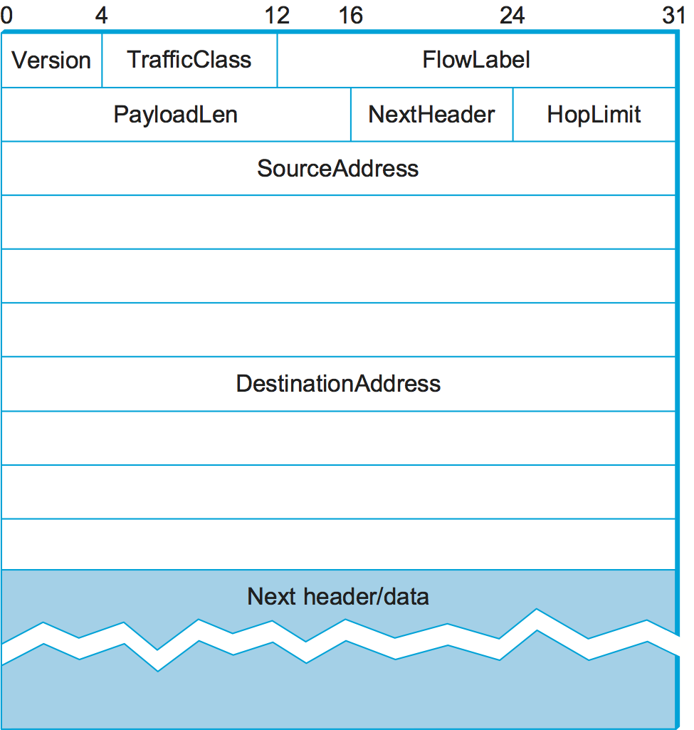
Figure 108. IPv6 packet header.

Finally, the bulk of the header is taken up with the source and destination addresses, each of which is 16 bytes (128 bits) long. Thus, the IPv6 header is always 40 bytes long. Considering that IPv6 addresses are four times longer than those of IPv4, this compares quite well with the IPv4 header, which is 20 bytes long in the absence of options.

The way that IPv6 handles options is quite an improvement over IPv4. In IPv4, if any options were present, every router had to parse the entire options field to see if any of the options were relevant. This is because the options were all buried at the end of the IP header, as an unordered collection of ‘(type, length, value)’ tuples. In contrast, IPv6 treats options as extension headers that must, if present, appear in a specific order. This means that each router can quickly determine if any of the options are relevant to it; in most cases, they will not be. Usually this can be determined by just looking at the NextHeader field. The end result is that option processing is much more efficient in IPv6, which is an important factor in router performance. In addition, the new formatting of options as extension headers means that they can be of arbitrary length, whereas in IPv4 they were limited to 44 bytes at most. We will see how some of the options are used below.

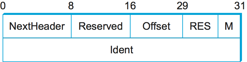
Figure 109. IPv6 fragmentation extension header.

Each option has its own type of extension header. The type of each extension header is identified by the value of the NextHeader field in the header that precedes it, and each extension header contains a NextHeader field to identify the header following it. The last extension header will be followed by a transport-layer header (e.g., TCP) and in this case the value of the NextHeader field is the same as the value of the Protocol field would be in an IPv4 header. Thus, the NextHeader field does double duty; it may either identify the type of extension header to follow, or, in the last extension header, it serves as a demux key to identify the higher-layer protocol running over IPv6.

Consider the example of the fragmentation header, shown in Figure 109. This header provides functionality similar to the fragmentation fields in the IPv4 header, but it is only present if fragmentation is necessary. Assuming it is the only extension header present, then the NextHeader field of the IPv6 header would contain the value 44, which is the value assigned to indicate the fragmentation header. The NextHeader field of the fragmentation header itself contains a value describing the header that follows it. Again, assuming no other extension headers are present, then the next header might be the TCP header, which results in NextHeader containing the value 6, just as the Protocol field would in IPv4. If the fragmentation header were followed by, say, an authentication header, then the fragmentation header’s NextHeader field would contain the value 51.

4.2.4 Advanced Capabilities

As mentioned at the beginning of this section, the primary motivation behind the development of IPv6 was to support the continued growth of the Internet. Once the IP header had to be changed for the sake of the addresses, however, the door was open for a wide variety of other changes, two of which we describe below. But IPv6 includes several additional features, most of which are covered elsewhere in this book; e.g., mobility, security, quality-of-service. It is interesting to note that, in most of these areas, the IPv4 and IPv6 capabilities have become virtually indistinguishable, so that the main driver for IPv6 remains the need for larger addresses.

Autoconfiguration

While the Internet’s growth has been impressive, one factor that has inhibited faster acceptance of the technology is the fact that getting connected to the Internet has typically required a fair amount of system administration expertise. In particular, every host that is connected to the Internet needs to be configured with a certain minimum amount of information, such as a valid IP address, a subnet mask for the link to which it attaches, and the address of a name server. Thus, it has not been possible to unpack a new computer and connect it to the Internet without some preconfiguration. One goal of IPv6, therefore, is to provide support for autoconfiguration, sometimes referred to as plug-and-play operation.

As we saw in the previous chapter, autoconfiguration is possible for IPv4, but it depends on the existence of a server that is configured to hand out addresses and other configuration information to Dynamic Host Configuration Protocol (DHCP) clients. The longer address format in IPv6 helps provide a useful, new form of autoconfiguration called stateless autoconfiguration, which does not require a server.

Recall that IPv6 unicast addresses are hierarchical, and that the least significant portion is the interface ID. Thus, we can subdivide the autoconfiguration problem into two parts:

1. Obtain an interface ID that is unique on the link to which the host is attached.

2. Obtain the correct address prefix for this subnet.

The first part turns out to be rather easy, since every host on a link must have a unique link-level address. For example, all hosts on an Ethernet have a unique 48-bit Ethernet address. This can be turned into a valid link-local use address by adding the appropriate prefix from Table 21 (1111 1110 10) followed by enough 0s to make up 128 bits. For some devices—for example, printers or hosts on a small routerless network that do not connect to any other networks—this address may be perfectly adequate. Those devices that need a globally valid address depend on a router on the same link to periodically advertise the appropriate prefix for the link. Clearly, this requires that the router be configured with the correct address prefix, and that this prefix be chosen in such a way that there is enough space at the end (e.g., 48 bits) to attach an appropriate link-level address.

The ability to embed link-level addresses as long as 48 bits into IPv6 addresses was one of the reasons for choosing such a large address size. Not only does 128 bits allow the embedding, but it leaves plenty of space for the multilevel hierarchy of addressing that we discussed above.

Source-Directed Routing

Another of IPv6’s extension headers is the routing header. In the absence of this header, routing for IPv6 differs very little from that of IPv4 under CIDR. The routing header contains a list of IPv6 addresses that represent nodes or topological areas that the packet should visit en route to its destination. A topological area may be, for example, a backbone provider’s network. Specifying that packets must visit this network would be a way of implementing provider selection on a packet-by-packet basis. Thus, a host could say that it wants some packets to go through a provider that is cheap, others through a provider that provides high reliability, and still others through a provider that the host trusts to provide security.

To provide the ability to specify topological entities rather than individual nodes, IPv6 defines an anycast address. An anycast address is assigned to a set of interfaces, and packets sent to that address will go to the “nearest” of those interfaces, with nearest being determined by the routing protocols. For example, all the routers of a backbone provider could be assigned a single anycast address, which would be used in the routing header.