4.4 Multiprotocol Label Switching
We continue our discussion of enhancements to IP by describing an addition to the Internet architecture that is very widely used but largely hidden from end users. The enhancement, called Multiprotocol Label Switching (MPLS), combines some of the properties of virtual circuits with the flexibility and robustness of datagrams. On the one hand, MPLS is very much associated with the Internet Protocol’s datagram-based architecture—it relies on IP addresses and IP routing protocols to do its job. On the other hand, MPLS-enabled routers also forward packets by examining relatively short, fixed-length labels, and these labels have local scope, just like in a virtual circuit network. It is perhaps this marriage of two seemingly opposed technologies that has caused MPLS to have a somewhat mixed reception in the Internet engineering community.
Before looking at how MPLS works, it is reasonable to ask “what is it good for?” Many claims have been made for MPLS, but there are three main things that it is used for today:
To enable IP capabilities on devices that do not have the capability to forward IP datagrams in the normal manner
To forward IP packets along explicit routes—precalculated routes that don’t necessarily match those that normal IP routing protocols would select
To support certain types of virtual private network services
It is worth noting that one of the original goals—improving performance—is not on the list. This has a lot to do with the advances that have been made in forwarding algorithms for IP routers in recent years and with the complex set of factors beyond header processing that determine performance.
The best way to understand how MPLS works is to look at some examples of its use. In the next three sections, we will look at examples to illustrate the three applications of MPLS mentioned above.
4.4.1 Destination-Based Forwarding
One of the earliest publications to introduce the idea of attaching labels to IP packets was a paper by Chandranmenon and Varghese that described an idea called threaded indices. A very similar idea is now implemented in MPLS-enabled routers. The following example shows how this idea works.
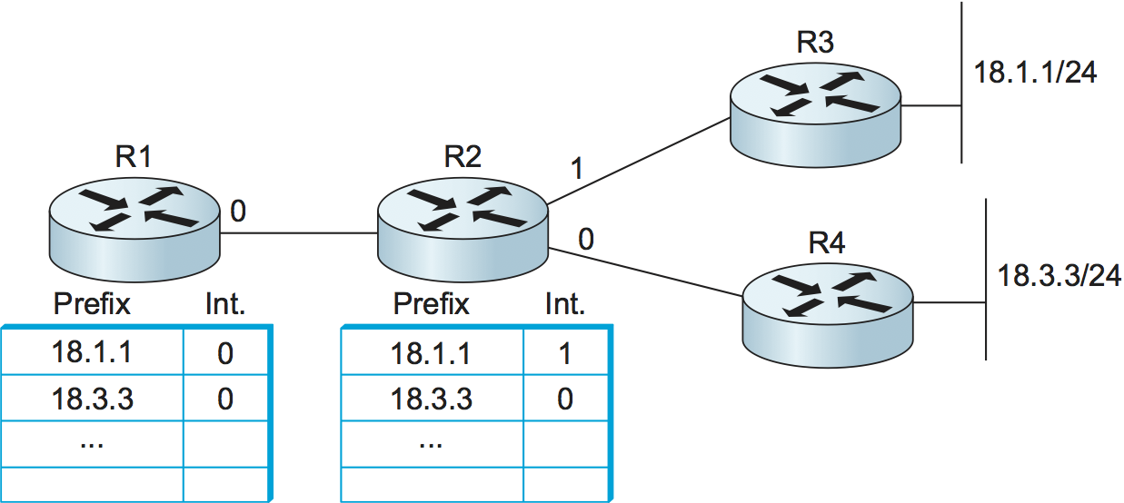
Figure 114. Routing tables in example network.
Consider the network in Figure 114. Each of
the two routers on the far right (R3 and R4) has one connected
network, with prefixes 18.1.1/24 and 18.3.3/24. The remaining
routers (R1 and R2) have routing tables that indicate which outgoing
interface each router would use when forwarding packets to one of
those two networks.
When MPLS is enabled on a router, the router allocates a label for
each prefix in its routing table and advertises both the label and the
prefix that it represents to its neighboring routers. This
advertisement is carried in the Label Distribution Protocol. This is
illustrated in Figure 115. Router R2 has
allocated the label value 15 for the prefix 18.1.1 and the
label value 16 for the prefix 18.3.3. These labels can be
chosen at the convenience of the allocating router and can be thought
of as indices into the routing table. After allocating the labels, R2
advertises the label bindings to its neighbors; in this case, we see
R2 advertising a binding between the label 15 and the prefix
18.1.1 to R1. The meaning of such an advertisement is that R2 has
said, in effect, “Please attach the label 15 to all packets sent
to me that are destined to prefix 18.1.1.” R1 stores the label in
a table alongside the prefix that it represents as the remote or
outgoing label for any packets that it sends to that prefix.
In Figure 115(c), we see another label
advertisement from router R3 to R2 for the prefix 18.1.1, and R2
places the remote label that it learned from R3 in the appropriate
place in its table.
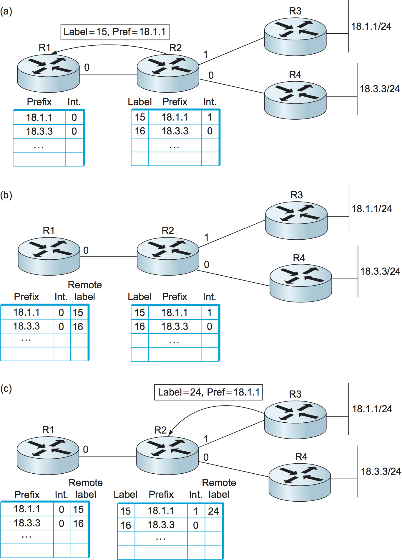
Figure 115. (a) R2 allocates labels and advertises bindings to R1. (b) R1 stores the received labels in a table. (c) R3 advertises another binding, and R2 stores the received label in a table.
At this point, we can look at what happens when a packet is forwarded in
this network. Suppose a packet destined to the IP address 18.1.1.5
arrives from the left to router R1. R1 in this case is referred to as a
Label Edge Router (LER); an LER performs a complete IP lookup on
arriving IP packets and then applies labels to them as a result of the
lookup. In this case, R1 would see that 18.1.1.5 matches the prefix
18.1.1 in its forwarding table and that this entry contains both an
outgoing interface and a remote label value. R1 therefore attaches the
remote label 15 to the packet before sending it.
When the packet arrives at R2, R2 looks only at the label in the packet,
not the IP address. The forwarding table at R2 indicates that packets
arriving with a label value of 15 should be sent out interface 1 and
that they should carry the label value 24, as advertised by router
R3. R2 therefore rewrites, or swaps, the label and forwards it on to R3.
What has been accomplished by all this application and swapping of labels? Observe that when R2 forwarded the packet in this example it never actually needed to examine the IP address. Instead, R2 looked only at the incoming label. Thus, we have replaced the normal IP destination address lookup with a label lookup. To understand why this is significant, it helps to recall that, although IP addresses are always the same length, IP prefixes are of variable length, and the IP destination address lookup algorithm needs to find the longest match—the longest prefix that matches the high order bits in the IP address of the packet being forwarded. By contrast, the label forwarding mechanism just described is an exact match algorithm. It is possible to implement a very simple exact match algorithm, for example, by using the label as an index into an array, where each element in the array is one line in the forwarding table.
Note that, while the forwarding algorithm has been changed from longest match to exact match, the routing algorithm can be any standard IP routing algorithm (e.g., OSPF). The path that a packet will follow in this environment is the exact same path that it would have followed if MPLS were not involved: the path chosen by the IP routing algorithms. All that has changed is the forwarding algorithm.
An important fundamental concept of MPLS is illustrated by this example. Every MPLS label is associated with a forwarding equivalence class (FEC)—a set of packets that are to receive the same forwarding treatment in a particular router. In this example, each prefix in the routing table is an FEC; that is, all packets that match the prefix 18.1.1—no matter what the low order bits of the IP address are—get forwarded along the same path. Thus, each router can allocate one label that maps to 18.1.1, and any packet that contains an IP address whose high order bits match that prefix can be forwarded using that label.
As we will see in the subsequent examples, FECs are a very powerful and flexible concept. FECs can be formed using almost any criteria; for example, all the packets corresponding to a particular customer could be considered to be in the same FEC.
Returning to the example at hand, we observe that changing the forwarding algorithm from normal IP forwarding to label swapping has an important consequence: Devices that previously didn’t know how to forward IP packets can be used to forward IP traffic in an MPLS network. The most notable early application of this result was to ATM switches, which can support MPLS without any changes to their forwarding hardware. ATM switches support the label-swapping forwarding algorithm just described, and by providing these switches with IP routing protocols and a method to distribute label bindings they could be turned into Label Switching Routers (LSRs)—devices that run IP control protocols but use the label switching forwarding algorithm. More recently, the same idea has been applied to optical switches.
Before we consider the purported benefits of turning an ATM switch into an LSR, we should tie up some loose ends. We have said that labels are “attached” to packets, but where exactly are they attached? The answer depends on the type of link on which packets are carried. Two common methods for carrying labels on packets are shown in Figure 116. When IP packets are carried as complete frames, as they are on most link types including Ethernet and PPP, the label is inserted as a “shim” between the layer 2 header and the IP (or other layer 3) header, as shown in the lower part of the figure. However, if an ATM switch is to function as an MPLS LSR, then the label needs to be in a place where the switch can use it, and that means it needs to be in the ATM cell header, exactly where one would normally find the virtual circuit identifier (VCI) and virtual path identifier (VPI) fields.
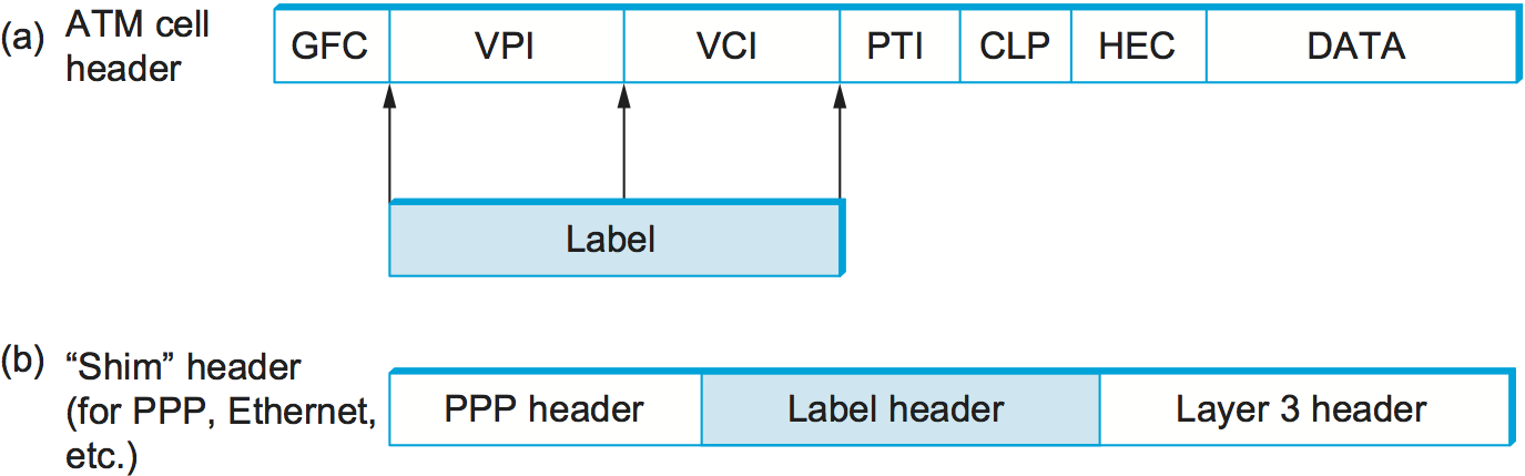
Figure 116. (a) Label on an ATM-encapsulated packet; (b) label on a frame-encapsulated packet.
Having now devised a scheme by which an ATM switch can function as an LSR, what have we gained? One thing to note is that we could now build a network that uses a mixture of conventional IP routers, label edge routers, and ATM switches functioning as LSRs, and they would all use the same routing protocols. To understand the benefits of using the same protocols, consider the alternative. In Figure 117(a), we see a set of routers interconnected by virtual circuits over an ATM network, a configuration called an overlay network. At one point in time, networks of this type were often built because commercially available ATM switches supported higher total throughput than routers. Today, networks like this are less common because routers have caught up with and even surpassed ATM switches. However, these networks still exist because of the significant installed base of ATM switches in network backbones, which in turn is partly a result of ATM’s ability to support a range of capabilities such as circuit emulation and virtual circuit services.
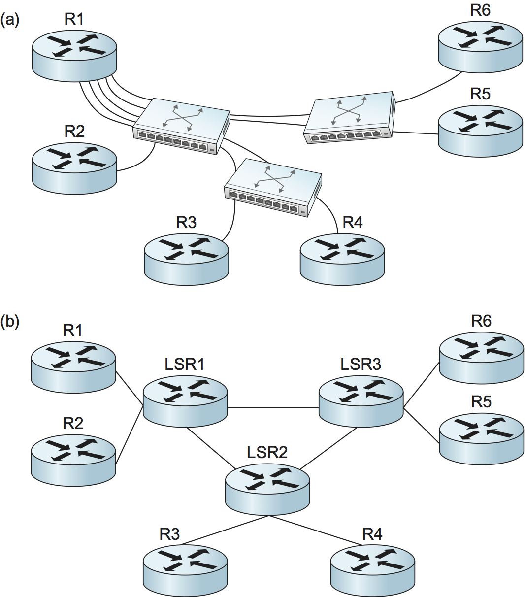
Figure 117. (a) Routers connect to each other using an overlay of virtual circuits. (b) Routers peer directly with LSRs.
In an overlay network, each router would potentially be connected to each of the other routers by a virtual circuit, but in this case for clarity we have just shown the circuits from R1 to all of its peer routers. R1 has five routing neighbors and needs to exchange routing protocol messages with all of them—we say that R1 has five routing adjacencies. By contrast, in Figure 117(b), the ATM switches have been replaced with LSRs. There are no longer virtual circuits interconnecting the routers. Thus, R1 has only one adjacency, with LSR1. In large networks, running MPLS on the switches leads to a significant reduction in the number of adjacencies that each router must maintain and can greatly reduce the amount of work that the routers have to do to keep each other informed of topology changes.
A second benefit of running the same routing protocols on edge routers and on the LSRs is that the edge routers now have a full view of the topology of the network. This means that if some link or node fails inside the network, the edge routers will have a better chance of picking a good new path than if the ATM switches rerouted the affected VCs without the knowledge of the edge routers.
Note that the step of “replacing” ATM switches with LSRs is actually achieved by changing the protocols running on the switches, but typically no change to the forwarding hardware is needed; that is, an ATM switch can often be converted to an MPLS LSR by upgrading only its software. Furthermore, an MPLS LSR might continue to support standard ATM capabilities at the same time as it runs the MPLS control protocols, in what is referred to as “ships in the night” mode.
The idea of running IP control protocols on devices that are unable to forward IP packets natively has been extended to Wavelength Division Multiplexing (WDM) and Time Division Multiplexing (TDM) networks (e.g., SONET). This is known as Generalized MPLS (GMPLS). Part of the motivation for GMPLS was to provide routers with topological knowledge of an optical network, just as in the ATM case. Even more important was the fact that there were no standard protocols for controlling optical devices, so MPLS proved to be a natural fit for that job.
4.4.2 Explicit Routing
IP has a source routing option, but it is not widely used for several reasons, including the fact that only a limited number of hops can be specified and because it is usual processed outside the “fast path” on most routers.
MPLS provides a convenient way to add capabilities similar to source-routing to IP networks, although the capability is more often referred to as explicit routing rather than source routing. One reason for the distinction is that it usually isn’t the real source of the packet that picks the route. More often it is one of the routers inside a service provider’s network. Figure 118 shows an example of how the explicit routing capability of MPLS might be applied. This sort of network is often called a fish network because of its shape (the routers R1 and R2 form the tail; R7 is at the head).
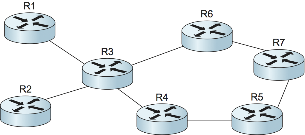
Figure 118. A network requiring explicit routing.
Suppose that the operator of the network in Figure 118 has determined that any traffic flowing from R1 to R7 should follow the path R1-R3-R6-R7 and that any traffic going from R2 to R7 should follow the path R2-R3-R4-R5-R7. One reason for such a choice would be to make good use of the capacity available along the two distinct paths from R3 to R7. We can think of the R1-to-R7 traffic as constituting one forwarding equivalence class, and the R2-to-R7 traffic constitutes a second FEC. Forwarding traffic in these two classes along different paths is difficult with normal IP routing, because R3 doesn’t normally look at where traffic came from in making its forwarding decisions.
Because MPLS uses label swapping to forward packets, it is easy enough to achieve the desired routing if the routers are MPLS enabled. If R1 and R2 attach distinct labels to packets before sending them to R3—thus identifying them as being in different FECs—then R3 can forward packets from R1 and R2 along different paths. The question that then arises is how do all the routers in the network agree on what labels to use and how to forward packets with particular labels? Clearly, we can’t use the same procedures as described in the preceding section to distribute labels, because those procedures establish labels that cause packets to follow the normal paths picked by IP routing, which is exactly what we are trying to avoid. Instead, a new mechanism is needed. It turns out that the protocol used for this task is the Resource Reservation Protocol (RSVP). For now it suffices to say that it is possible to send an RSVP message along an explicitly specified path (e.g., R1-R3-R6-R7) and use it to set up label forwarding table entries all along that path. This is very similar to the process of establishing a virtual circuit.
One of the applications of explicit routing is traffic engineering, which refers to the task of ensuring that sufficient resources are available in a network to meet the demands placed on it. Controlling exactly which paths the traffic flows on is an important part of traffic engineering. Explicit routing can also help to make networks more resilient in the face of failure, using a capability called fast reroute. For example, it is possible to precalculate a path from router A to router B that explicitly avoids a certain link L. In the event that link L fails, router A could send all traffic destined to B down the precalculated path. The combination of precalculation of the backup path and the explicit routing of packets along the path means that A doesn’t need to wait for routing protocol packets to make their way across the network or for routing algorithms to be executed by various other nodes in the network. In certain circumstances, this can significantly reduce the time taken to reroute packets around a point of failure.
One final point to note about explicit routing is that explicit routes need not be calculated by a network operator as in the above example. Routers can use various algorithms to calculate explicit routes automatically. The most common of these is constrained shortest path first (CSPF), which is a link-state algorithm, but which also takes various constraints into account. For example, if it was required to find a path from R1 to R7 that could carry an offered load of 100 Mbps, we could say that the constraint is that each link must have at least 100 Mbps of available capacity. CSPF addresses this sort of problem.
4.4.3 Virtual Private Networks and Tunnels
One way to build virtual private networks (VPNs) is to use tunnels. It turns out that MPLS can be thought of as a way to build tunnels, and this makes it suitable for building VPNs of various types.
The simplest form of MPLS VPN to understand is a layer 2 VPN. In this type of VPN, MPLS is used to tunnel layer 2 data (such as Ethernet frames or ATM cells) across a network of MPLS-enabled routers. One reason for tunnels is to provide some sort of network service (such as multicast) that is not supported by some routers in the network. The same logic applies here: IP routers are not ATM switches, so you cannot provide an ATM virtual circuit service across a network of conventional routers. However, if you had a pair of routers interconnected by a tunnel, they could send ATM cells across the tunnel and emulate an ATM circuit. The term for this technique within the IETF is pseudowire emulation. Figure 119 illustrates the idea.
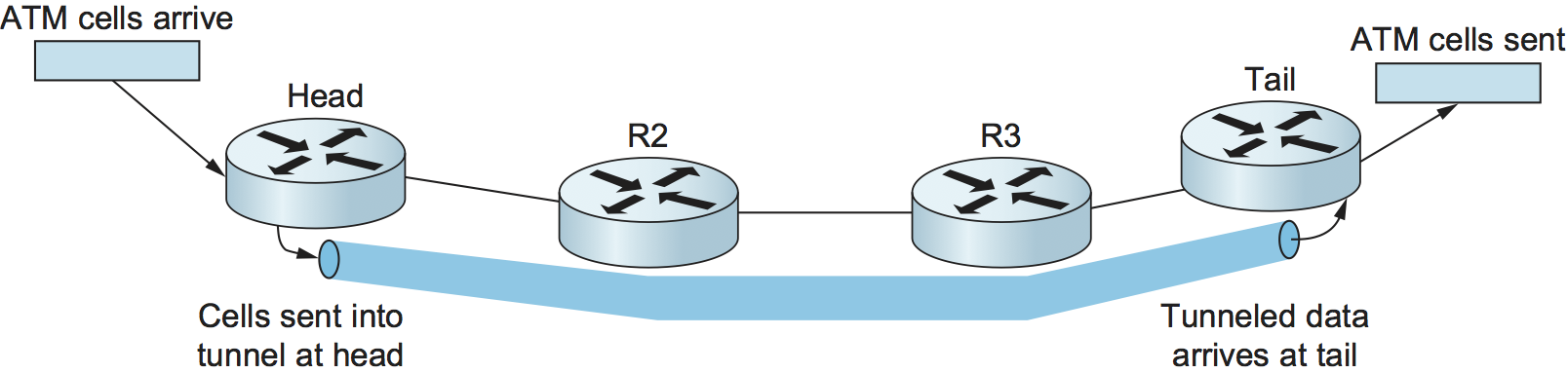
Figure 119. An ATM circuit is emulated by a tunnel.
We have already seen how IP tunnels are built: The router at the entrance of the tunnel wraps the data to be tunneled in an IP header (the tunnel header), which represents the address of the router at the far end of the tunnel and sends the data like any other IP packet. The receiving router receives the packet with its own address in the header, strips the tunnel header, and finds the data that was tunneled, which it then processes. Exactly what it does with that data depends on what it is. For example, if it were another IP packet, it would then be forwarded on like a normal IP packet. However, it need not be an IP packet, as long as the receiving router knows what to do with non-IP packets. We’ll return to the issue of how to handle non-IP data in a moment.
An MPLS tunnel is not too different from an IP tunnel, except that the
tunnel header consists of an MPLS header rather than an IP header.
Looking back to our first example, in Figure 115, we saw that router R1 attached a label (15) to
every packet that it sent towards prefix 18.1.1. Such a packet would
then follow the path R1-R2-R3, with each router in the path examining
only the MPLS label. Thus, we observe that there was no requirement
that R1 only send IP packets along this path—any data could be wrapped
up in the MPLS header and it would follow the same path, because the
intervening routers never look beyond the MPLS header. In this regard,
an MPLS header is just like an IP tunnel header (except only 4 bytes
long instead of 20 bytes). The only issue with sending non-IP traffic
along a tunnel, MPLS or otherwise, is what to do with non-IP traffic
when it reaches the end of the tunnel. The general solution is to
carry some sort of demultiplexing identifier in the tunnel payload
that tells the router at the end of the tunnel what to do. It turns
out that an MPLS label is a perfect fit for such an identifier. An
example will make this clear.
Let’s assume we want to tunnel ATM cells from one router to another across a network of MPLS-enabled routers, as in Figure 119. Further, we assume that the goal is to emulate an ATM virtual circuit; that is, cells arrive at the entrance, or head, of the tunnel on a certain input port with a certain VCI and should leave the tail end of the tunnel on a certain output port and potentially different VCI. This can be accomplished by configuring the head and tail routers as follows:
The head router needs to be configured with the incoming port, the incoming VCI, the demultiplexing label for this emulated circuit, and the address of the tunnel end router.
The tail router needs to be configured with the outgoing port, the outgoing VCI, and the demultiplexing label.
Once the routers are provided with this information, we can see how an ATM cell would be forwarded. Figure 120 illustrates the steps.
An ATM cell arrives on the designated input port with the appropriate VCI value (101 in this example).
The head router attaches the demultiplexing label that identifies the emulated circuit.
The head router then attaches a second label, which is the tunnel label that will get the packet to the tail router. This label is learned by mechanisms just like those described elsewhere in this section.
Routers between the head and tail forward the packet using only the tunnel label.
The tail router removes the tunnel label, finds the demultiplexing label, and recognizes the emulated circuit.
The tail router modifies the ATM VCI to the correct value (202 in this case) and sends it out the correct port.
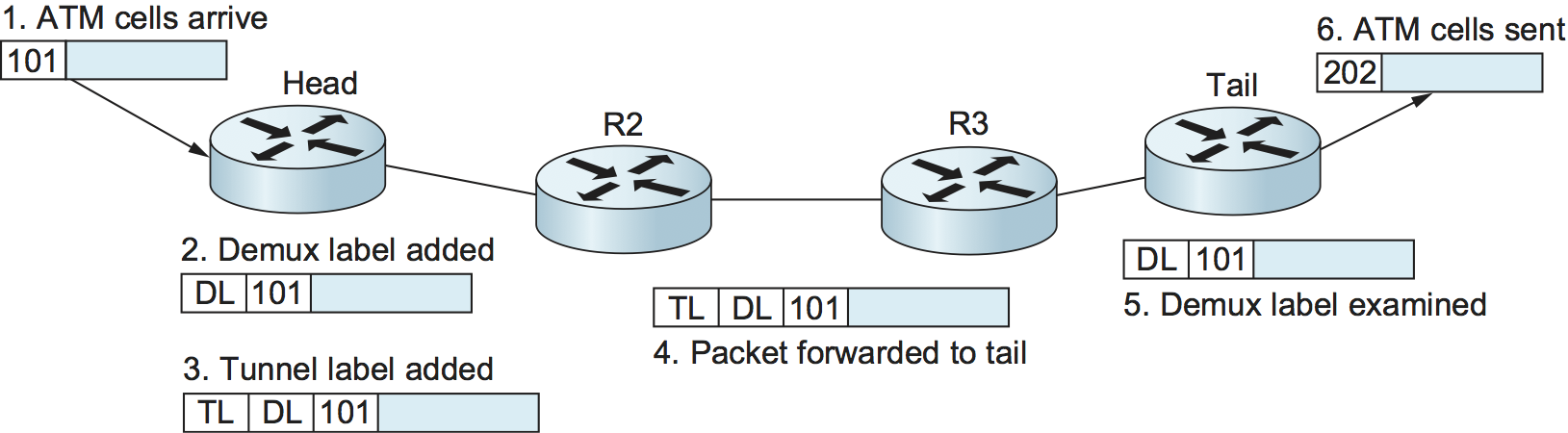
Figure 120. Forward ATM cells along a tunnel.
One item in this example that might be surprising is that the packet has two labels attached to it. This is one of the interesting features of MPLS—labels may be stacked on a packet to any depth. This provides some useful scaling capabilities. In this example, it allows a single tunnel to carry a potentially large number of emulated circuits.
The same techniques described here can be applied to emulate many other layer 2 services, including Frame Relay and Ethernet. It is worth noting that virtually identical capabilities can be provided using IP tunnels; the main advantage of MPLS here is the shorter tunnel header.
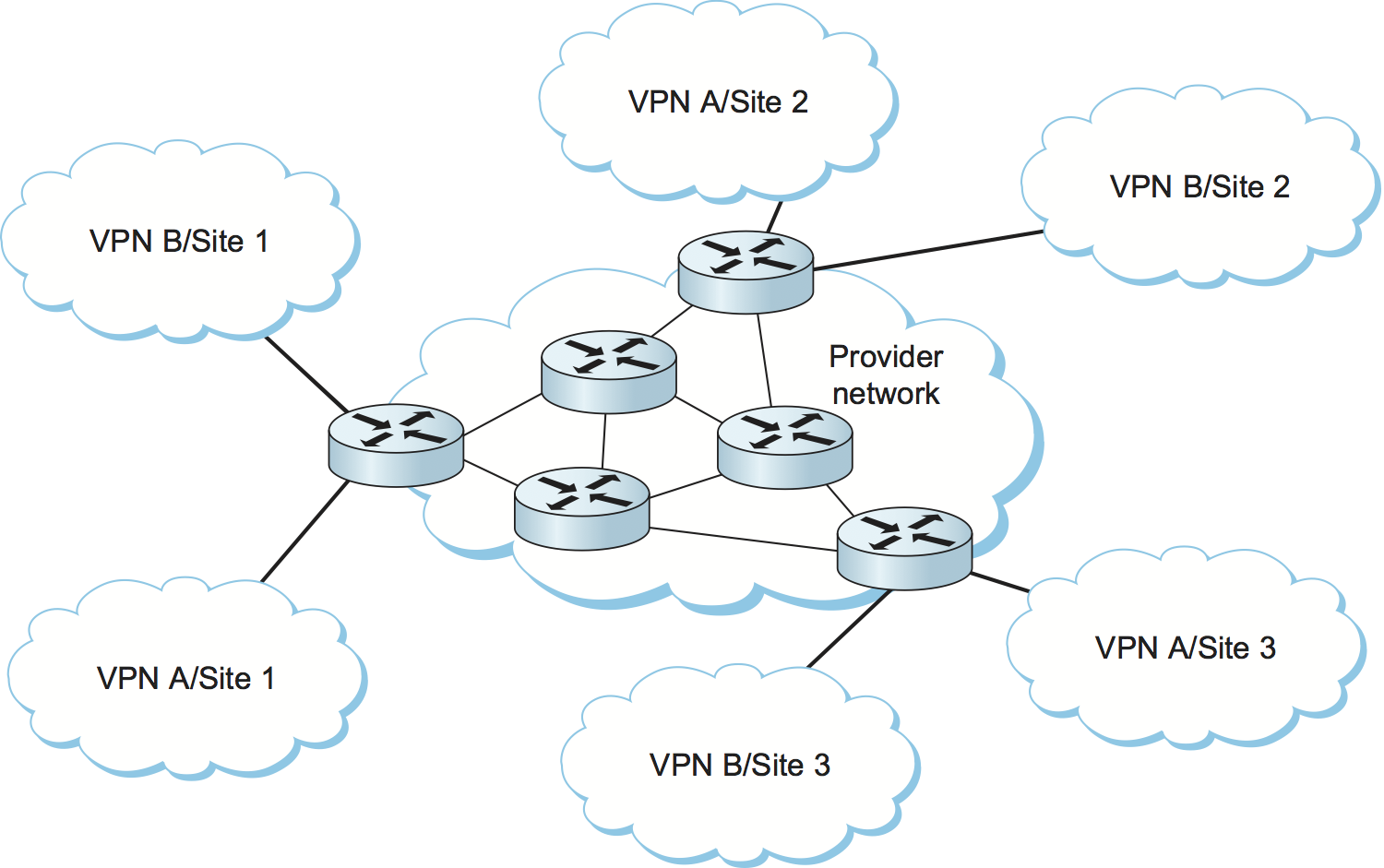
Figure 121. Example of a layer 3 VPN. Customers A and B each obtain a virtually private IP service from a single provider.
Before MPLS was used to tunnel layer 2 services, it was also being used to support layer 3 VPNs. We won’t go into the details of layer 3 VPNs, which are quite complex, but we will note that they represent one of the most popular uses of MPLS today. Layer 3 VPNs also use stacks of MPLS labels to tunnel packets across an IP network. However, the packets that are tunneled are themselves IP packets—hence, the name layer 3 VPNs. In a layer 3 VPN, a single service provider operates a network of MPLS-enabled routers and provides a “virtually private” IP network service to any number of distinct customers. That is, each customer of the provider has some number of sites, and the service provider creates the illusion for each customer that there are no other customers on the network. The customer sees an IP network interconnecting his own sites and no other sites. This means that each customer is isolated from all other customers in terms of both routing and addressing. Customer A can’t sent packets directly to customer B, and vice versa. Customer A can even use IP addresses that have also been used by customer B. The basic idea is illustrated in Figure 121. As in layer 2 VPNs, MPLS is used to tunnel packets from one site to another; however, the configuration of the tunnels is performed automatically by some fairly elaborate use of BGP, which is beyond the scope of this book.
Customer A in fact usually can send data to customer B in some restricted way. Most likely, both customer A and customer B have some connection to the global Internet, and thus it is probably possible for customer A to send email messages, for example, to the mail server inside customer B’s network. The “privacy” offered by a VPN prevents customer A from having unrestricted access to all the machines and subnets inside customer B’s network.
In summary, MPLS is a rather versatile tool that has been applied to a wide range of different networking problems. It combines the label-swapping forwarding mechanism that is normally associated with virtual circuit networks with the routing and control protocols of IP datagram networks to produce a class of network that is somewhere between the two conventional extremes. This extends the capabilities of IP networks to enable, among other things, more precise control of routing and the support of a range of VPN services.