7.2 Multimedia Data
Multimedia data, comprised of audio, video, and still images, now makes up the majority of traffic on the Internet. Part of what has made the widespread transmission of multimedia across networks possible is advances in compression technology. Because multimedia data is consumed mostly by humans using their senses—vision and hearing—and processed by the human brain, there are unique challenges to compressing it. You want to try to keep the information that is most important to a human, while getting rid of anything that doesn’t improve the human’s perception of the visual or auditory experience. Hence, both computer science and the study of human perception come into play. In this section, we’ll look at some of the major efforts in representing and compressing multimedia data.
The uses of compression are not limited to multimedia data of course—for
example, you may well have used a utility like zip or compress
to compress files before sending them over a network, or to uncompress a
data file after downloading. It turns out that the techniques used for
compressing data—which are typically lossless, because most people
don’t like to lose data from a file—also show up as part of the solution
for multimedia compression. In contrast, lossy compression, commonly
used for multimedia data, does not promise that the data received is
exactly the same as the data sent. As noted above, this is because
multimedia data often contains information that is of little utility to
the human who receives it. Our senses and brains can only perceive so
much detail. They are also very good at filling in missing pieces and
even correcting some errors in what we see or hear. And, lossy
algorithms typically achieve much better compression ratios than do
their lossless counterparts; they can be an order of magnitude better or
more.
To get a sense of how important compression has been to the spread of networked multimedia, consider the following example. A high-definition TV screen has something like 1080 × 1920 pixels, each of which has 24 bits of color information, so each frame is
1080 × 1920 × 24 = 50 Mb
so if you want to send 24 frames per second, that would be over 1 Gbps. That’s more than most Internet users have access to. By contrast, modern compression techniques can get a reasonably high-quality HDTV signal down to the range of 10 Mbps, a two order of magnitude reduction and well within the reach of most broadband users. Similar compression gains apply to lower quality video such as YouTube clips—Web video could never have reached its current popularity without compression to make all those entertaining videos fit within the bandwidth of today’s networks.
Compression techniques as applied to multimedia have been an area of great innovation, particularly lossy compression. Lossless techniques also have an important role to play, however. Indeed, most of the lossy techniques include some steps that are lossless, so we begin our discussion with an overview of lossless compression.
7.2.1 Lossless Compression Techniques
In many ways, compression is inseparable from data encoding. When thinking about how to encode a piece of data in a set of bits, we might just as well think about how to encode the data in the smallest set of bits possible. For example, if you have a block of data that is made up of the 26 symbols A through Z, and if all of these symbols have an equal chance of occurring in the data block you are encoding, then encoding each symbol in 5 bits is the best you can do (since 25 = 32 is the lowest power of 2 above 26). If, however, the symbol R occurs 50% of the time, then it would be a good idea to use fewer bits to encode the R than any of the other symbols. In general, if you know the relative probability that each symbol will occur in the data, then you can assign a different number of bits to each possible symbol in a way that minimizes the number of bits it takes to encode a given block of data. This is the essential idea of Huffman codes, one of the important early developments in data compression.
Run Length Encoding
Run length encoding (RLE) is a compression technique with a brute-force
simplicity. The idea is to replace consecutive occurrences of a given
symbol with only one copy of the symbol, plus a count of how many times
that symbol occurs—hence, the name run length. For example, the string
AAABBCDDDD would be encoded as 3A2B1C4D.
RLE turns out to be useful for compressing some classes of images. It can be used in this context by comparing adjacent pixel values and then encoding only the changes. For images that have large homogeneous regions, this technique is quite effective. For example, it is not uncommon that RLE can achieve compression ratios on the order of 8-to-1 for scanned text images. RLE works well on such files because they often contain a large amount of white space that can be removed. For those old enough to remember the technology, RLE was the key compression algorithm used to transmit faxes. However, for images with even a small degree of local variation, it is not uncommon for compression to actually increase the image byte size, since it takes 2 bytes to represent a single symbol when that symbol is not repeated.
Differential Pulse Code Modulation
Another simple lossless compression algorithm is Differential Pulse Code
Modulation (DPCM). The idea here is to first output a reference symbol
and then, for each symbol in the data, to output the difference between
that symbol and the reference symbol. For example, using symbol A as the
reference symbol, the string AAABBCDDDD would be encoded as
A0001123333 because A is the same as the reference symbol, B has a
difference of 1 from the reference symbol, and so on. Note that this
simple example does not illustrate the real benefit of DPCM, which is
that when the differences are small they can be encoded with fewer bits
than the symbol itself. In this example, the range of differences, 0-3,
can be represented with 2 bits each, rather than the 7 or 8 bits
required by the full character. As soon as the difference becomes too
large, a new reference symbol is selected.
DPCM works better than RLE for most digital imagery, since it takes advantage of the fact that adjacent pixels are usually similar. Due to this correlation, the dynamic range of the differences between the adjacent pixel values can be significantly less than the dynamic range of the original image, and this range can therefore be represented using fewer bits. Using DPCM, we have measured compression ratios of 1.5-to-1 on digital images. DPCM also works on audio, because adjacent samples of an audio waveform are likely to be close in value.
A slightly different approach, called delta encoding, simply encodes a
symbol as the difference from the previous one. Thus, for example,
AAABBCDDDD would be represented as A001011000. Note that delta
encoding is likely to work well for encoding images where adjacent
pixels are similar. It is also possible to perform RLE after delta
encoding, since we might find long strings of 0s if there are many
similar symbols next to each other.
Dictionary-Based Methods
The final lossless compression method we consider is the
dictionary-based approach, of which the Lempel-Ziv (LZ) compression
algorithm is the best known. The Unix compress and gzip
commands use variants of the LZ algorithm.
The idea of a dictionary-based compression algorithm is to build a
dictionary (table) of variable-length strings (think of them as common
phrases) that you expect to find in the data and then to replace each of
these strings when it appears in the data with the corresponding index
to the dictionary. For example, instead of working with individual
characters in text data, you could treat each word as a string and
output the index in the dictionary for that word. To further elaborate
on this example, the word compression has the index 4978 in one
particular dictionary; it is the 4978th word in
/usr/share/dict/words. To compress a body of
text, each time the string “compression” appears, it would be replaced
by 4978. Since this particular dictionary has just over 25,000 words in
it, it would take 15 bits to encode the index, meaning that the string
“compression” could be represented in 15 bits rather than the 77 bits
required by 7-bit ASCII. This is a compression ratio of 5-to-1! At
another data point, we were able to get a 2-to-1 compression ratio when
we applied the compress command to the source code for the protocols
described in this book.
Of course, this leaves the question of where the dictionary comes from. One option is to define a static dictionary, preferably one that is tailored for the data being compressed. A more general solution, and the one used by LZ compression, is to adaptively define the dictionary based on the contents of the data being compressed. In this case, however, the dictionary constructed during compression has to be sent along with the data so that the decompression half of the algorithm can do its job. Exactly how you build an adaptive dictionary has been a subject of extensive research.
7.2.2 Image Representation and Compression (GIF, JPEG)
Given the ubiquitous use of digital imagery—this use was spawned by the invention of graphical displays, not high-speed networks—the need for standard representation formats and compression algorithms for digital imagery data has become essential. In response to this need, the ISO defined a digital image format known as JPEG, named after the Joint Photographic Experts Group that designed it. (The “Joint” in JPEG stands for a joint ISO/ITU effort.) JPEG is the most widely used format for still images in use today. At the heart of the definition of the format is a compression algorithm, which we describe below. Many techniques used in JPEG also appear in MPEG, the set of standards for video compression and transmission created by the Moving Picture Experts Group.
Before delving into the details of JPEG, we observe that there are quite a few steps to get from a digital image to a compressed representation of that image that can be transmitted, decompressed, and displayed correctly by a receiver. You probably know that digital images are made up of pixels (hence, the megapixels quoted in smartphone camera advertisements). Each pixel represents one location in the two-dimensional grid that makes up the image, and for color images each pixel has some numerical value representing a color. There are lots of ways to represent colors, referred to as color spaces; the one most people are familiar with is RGB (red, green, blue). You can think of color as being a three dimensional quantity—you can make any color out of red, green, and blue light in different amounts. In a three-dimensional space, there are lots of different, valid ways to describe a given point (consider Cartesian and polar coordinates, for example). Similarly, there are various ways to describe a color using three quantities, and the most common alternative to RGB is YUV. The Y is luminance, roughly the overall brightness of the pixel, and U and V contain chrominance, or color information. Confoundingly, there are a few different variants of the YUV color space as well. More on this in a moment.
The significance of this discussion is that the encoding and transmission of color images (either still or moving) requires agreement between the two ends on the color space. Otherwise, of course, you’d end up with different colors being displayed by the receiver than were captured by the sender. Hence, agreeing on a color space definition (and perhaps a way to communicate which particular space is in use) is part of the definition of any image or video format.
Let’s look at the example of the Graphical Interchange Format (GIF). GIF uses the RGB color space and starts out with 8 bits to represent each of the three dimensions of color for a total of 24 bits. Rather than sending those 24 bits per pixel, however, GIF first reduces 24-bit color images to 8-bit color images. This is done by identifying the colors used in the picture, of which there will typically be considerably fewer than 224, and then picking the 256 colors that most closely approximate the colors used in the picture. There might be more than 256 colors, however, so the trick is to try not to distort the color too much by picking 256 colors such that no pixel has its color changed too much.
The 256 colors are stored in a table, which can be indexed with an 8-bit number, and the value for each pixel is replaced by the appropriate index. Note that this is an example of lossy compression for any picture with more than 256 colors. GIF then runs an LZ variant over the result, treating common sequences of pixels as the strings that make up the dictionary—a lossless operation. Using this approach, GIF is sometimes able to achieve compression ratios on the order of 10:1, but only when the image consists of a relatively small number of discrete colors. Graphical logos, for example, are handled well by GIF. Images of natural scenes, which often include a more continuous spectrum of colors, cannot be compressed at this ratio using GIF. It is also not too hard for a human eye to detect the distortion caused by the lossy color reduction of GIF in some cases.
The JPEG format is considerably more well suited to photographic images, as you would hope given the name of the group that created it. JPEG does not reduce the number of colors like GIF. Instead, JPEG starts off by transforming the RGB colors (which are what you usually get out of a digital camera) to the YUV space. The reason for this has to do with the way the eye perceives images. There are receptors in the eye for brightness, and separate receptors for color. Because we’re very good at perceiving variations in brightness, it makes sense to spend more bits on transmitting brightness information. Since the Y component of YUV is, roughly, the brightness of the pixel, we can compress that component separately, and less aggressively, from the other two (chrominance) components.
As noted above, YUV and RGB are alternative ways to describe a point in a 3-dimensional space, and it’s possible to convert from one color space to another using linear equations. For one YUV space that is commonly used to represent digital images, the equations are:
Y = 0.299R + 0.587G + 0.114B
U = (B-Y) x 0.565
V =  (R-Y) x 0.713
The exact values of the constants here are not important, as long as the encoder and decoder agree on what they are. (The decoder will have to apply the inverse transformations to recover the RGB components needed to drive a display.) The constants are, however, carefully chosen based on the human perception of color. You can see that Y, the luminance, is a sum of the red, green, and blue components, while U and V are color difference components. U represents the difference between the luminance and blue, and V the difference between luminance and red. You may notice that setting R, G, and B to their maximum values (which would be 255 for 8-bit representations) will also produce a value of Y=255 while U and V in this case would be zero. That is, a fully white pixel is (255,255,255) in RGB space and (255,0,0) in YUV space.
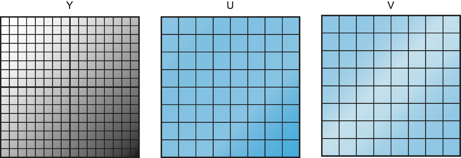
Figure 189. Subsampling the U and V components of an image.
Once the image has been transformed into YUV space, we can now think about compressing each of the three components separately. We want to be more aggressive in compressing the U and V components, to which human eyes are less sensitive. One way to compress the U and V components is to subsample them. The basic idea of subsampling is to take a number of adjacent pixels, calculate the average U or V value for that group of pixels, and transmit that, rather than sending the value for every pixel. Figure 189 illustrates the point. The luminance (Y) component is not subsampled, so the Y value of all the pixels will be transmitted, as indicated by the 16 × 16 grid of pixels on the left. In the case of U and V, we treat each group of four adjacent pixels as a group, calculate the average of the U or V value for that group, and transmit that. Hence, we end up with an 8 × 8 grid of U and V values to transmit. Thus, in this example, for every four pixels, we transmit six values (four Y and one each of U and V) rather than the original 12 values (four each for all three components), for a 50% reduction in information.
It’s worth noting that you could be either more or less aggressive in the subsampling, with corresponding increases in compression and decreases in quality. The subsampling approach shown here, in which chrominance is subsampled by a factor of two in both horizontal and vertical directions (and which goes by the identification 4:2:0), happens to match the most common approach used for both JPEG and MPEG.
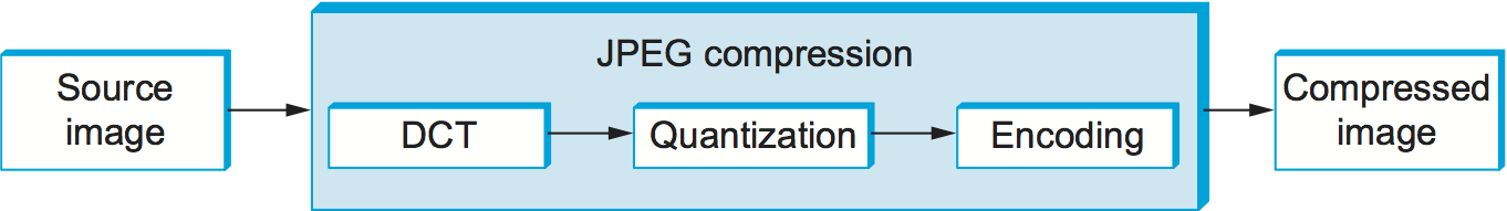
Figure 190. Block diagram of JPEG compression.
Once subsampling is done, we now have three grids of pixels to deal with, and each one is dealt with separately. JPEG compression of each component takes place in three phases, as illustrated in Figure 190. On the compression side, the image is fed through these three phases one 8 × 8 block at a time. The first phase applies the discrete cosine transform (DCT) to the block. If you think of the image as a signal in the spatial domain, then DCT transforms this signal into an equivalent signal in the spatial frequency domain. This is a lossless operation but a necessary precursor to the next, lossy step. After the DCT, the second phase applies a quantization to the resulting signal and, in so doing, loses the least significant information contained in that signal. The third phase encodes the final result, but in so doing also adds an element of lossless compression to the lossy compression achieved by the first two phases. Decompression follows these same three phases, but in reverse order.
DCT Phase
DCT is a transformation closely related to the fast Fourier transform (FFT). It takes an 8 × 8 matrix of pixel values as input and outputs an 8 × 8 matrix of frequency coefficients. You can think of the input matrix as a 64-point signal that is defined in two spatial dimensions (x and y); DCT breaks this signal into 64 spatial frequencies. To get an intuitive feel for spatial frequency, imagine yourself moving across a picture in, say, the x direction. You would see the value of each pixel varying as some function of x. If this value changes slowly with increasing x, then it has a low spatial frequency; if it changes rapidly, it has a high spatial frequency. So the low frequencies correspond to the gross features of the picture, while the high frequencies correspond to fine detail. The idea behind the DCT is to separate the gross features, which are essential to viewing the image, from the fine detail, which is less essential and, in some cases, might be barely perceived by the eye.
DCT, along with its inverse, which recovers the original pixels and during decompression, are defined by the following formulas:
where \(C(x) = 1/\sqrt{2}\) when \(x=0\) and \(1\) when \(x>0\), and \(pixel(x,y)\) is the grayscale value of the pixel at position (x,y) in the 8 × 8 block being compressed; N = 8 in this case.
The first frequency coefficient, at location (0,0) in the output matrix, is called the DC coefficient. Intuitively, we can see that the DC coefficient is a measure of the average value of the 64 input pixels. The other 63 elements of the output matrix are called the AC coefficients. They add the higher-spatial-frequency information to this average value. Thus, as you go from the first frequency coefficient toward the 64th frequency coefficient, you are moving from low-frequency information to high-frequency information, from the broad strokes of the image to finer and finer detail. These higher-frequency coefficients are increasingly unimportant to the perceived quality of the image. It is the second phase of JPEG that decides which portion of which coefficients to throw away.
Quantization Phase
The second phase of JPEG is where the compression becomes lossy. DCT does not itself lose information; it just transforms the image into a form that makes it easier to know what information to remove. (Although not lossy, per se, there is of course some loss of precision during the DCT phase because of the use of fixed-point arithmetic.) Quantization is easy to understand—it’s simply a matter of dropping the insignificant bits of the frequency coefficients.
To see how the quantization phase works, imagine that you want to compress some whole numbers less than 100, such as 45, 98, 23, 66, and 7. If you decided that knowing these numbers truncated to the nearest multiple of 10 is sufficient for your purposes, then you could divide each number by the quantum 10 using integer arithmetic, yielding 4, 9, 2, 6, and 0. These numbers can each be encoded in 4 bits rather than the 7 bits needed to encode the original numbers.
Quantum |
|||||||
|---|---|---|---|---|---|---|---|
3 |
5 |
7 |
9 |
11 |
13 |
15 |
17 |
5 |
7 |
9 |
11 |
13 |
15 |
17 |
19 |
7 |
9 |
11 |
13 |
15 |
17 |
19 |
21 |
9 |
11 |
13 |
15 |
17 |
19 |
21 |
23 |
11 |
13 |
15 |
17 |
19 |
21 |
23 |
25 |
13 |
15 |
17 |
19 |
21 |
23 |
25 |
27 |
15 |
17 |
19 |
21 |
23 |
25 |
27 |
29 |
17 |
19 |
21 |
23 |
25 |
27 |
29 |
31 |
Rather than using the same quantum for all 64 coefficients, JPEG uses
a quantization table that gives the quantum to use for each of the
coefficients, as specified in the formula given below. You can think
of this table (Quantum) as a parameter that can be set to control
how much information is lost and, correspondingly, how much
compression is achieved. In practice, the JPEG standard specifies a
set of quantization tables that have proven effective in compressing
digital images; an example quantization table is given in
Table 24. In tables like this one, the low
coefficients have a quantum close to 1 (meaning that little
low-frequency information is lost) and the high coefficients have
larger values (meaning that more high-frequency information is
lost). Notice that as a result of such quantization tables many of the
high-frequency coefficients end up being set to 0 after quantization,
making them ripe for further compression in the third phase.
The basic quantization equation is
QuantizedValue(i,j) = IntegerRound(DCT(i,j)/Quantum(i,j))
where
IntegerRound(x) =
    Floor(x + 0.5) if x >= 0
    Floor(x - 0.5) if x < 0
Decompression is then simply defined as
DCT(i,j) = QuantizedValue(i,j) x Quantum(i,j)
For example, if the DC coefficient (i.e., DCT(0,0)) for a particular block was equal to 25, then the quantization of this value using Table 24 would result in
Floor(25/3+0.5) = 8
During decompression, this coefficient would then be restored as 8 × 3 = 24.
Encoding Phase
The final phase of JPEG encodes the quantized frequency coefficients in a compact form. This results in additional compression, but this compression is lossless. Starting with the DC coefficient in position (0,0), the coefficients are processed in the zigzag sequence shown in Figure 191. Along this zigzag, a form of run length encoding is used—RLE is applied to only the 0 coefficients, which is significant because many of the later coefficients are 0. The individual coefficient values are then encoded using a Huffman code. (The JPEG standard allows the implementer to use an arithmetic coding instead of the Huffman code.)
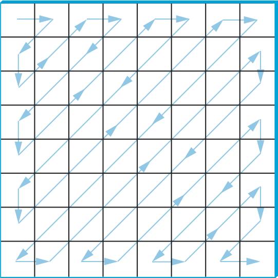
Figure 191. Zigzag traversal of quantized frequency coefficients.
In addition, because the DC coefficient contains a large percentage of the information about the 8 × 8 block from the source image, and images typically change slowly from block to block, each DC coefficient is encoded as the difference from the previous DC coefficient. This is the delta encoding approach described in a later section.
JPEG includes a number of variations that control how much compression you achieve versus the fidelity of the image. This can be done, for example, by using different quantization tables. These variations, plus the fact that different images have different characteristics, make it impossible to say with any precision the compression ratios that can be achieved with JPEG. Ratios of 30:1 are common, and higher ratios are certainly possible, but artifacts (noticeable distortion due to compression) become more severe at higher ratios.
7.2.3 Video Compression (MPEG)
We now turn our attention to the MPEG format, named after the Moving Picture Experts Group that defined it. To a first approximation, a moving picture (i.e., video) is simply a succession of still images—also called frames or pictures—displayed at some video rate. Each of these frames can be compressed using the same DCT-based technique used in JPEG. Stopping at this point would be a mistake, however, because it fails to remove the interframe redundancy present in a video sequence. For example, two successive frames of video will contain almost identical information if there is not much motion in the scene, so it would be unnecessary to send the same information twice. Even when there is motion, there may be plenty of redundancy since a moving object may not change from one frame to the next; in some cases, only its position changes. MPEG takes this interframe redundancy into consideration. MPEG also defines a mechanism for encoding an audio signal with the video, but we consider only the video aspect of MPEG in this section.
Frame Types
MPEG takes a sequence of video frames as input and compresses them into three types of frames, called I frames (intrapicture), P frames (predicted picture), and B frames (bidirectional predicted picture). Each frame of input is compressed into one of these three frame types. I frames can be thought of as reference frames; they are self-contained, depending on neither earlier frames nor later frames. To a first approximation, an I frame is simply the JPEG compressed version of the corresponding frame in the video source. P and B frames are not self-contained; they specify relative differences from some reference frame. More specifically, a P frame specifies the differences from the previous I frame, while a B frame gives an interpolation between the previous and subsequent I or P frames.
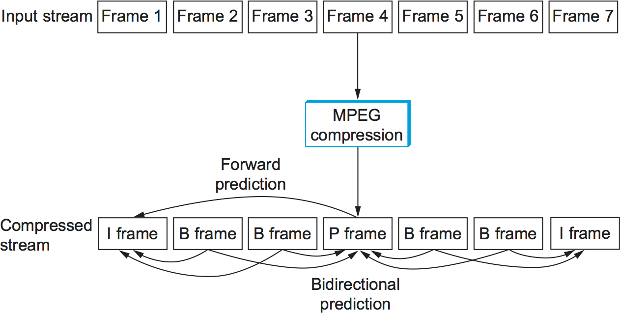
Figure 192. Sequence of I, P, and B frames generated by MPEG.
Figure 192 illustrates a sequence of seven video frames that, after being compressed by MPEG, result in a sequence of I, P, and B frames. The two I frames stand alone; each can be decompressed at the receiver independently of any other frames. The P frame depends on the preceding I frame; it can be decompressed at the receiver only if the preceding I frame also arrives. Each of the B frames depends on both the preceding I or P frame and the subsequent I or P frame. Both of these reference frames must arrive at the receiver before MPEG can decompress the B frame to reproduce the original video frame.
Note that, because each B frame depends on a later frame in the sequence, the compressed frames are not transmitted in sequential order. Instead, the sequence I B B P B B I shown in Figure 192 is transmitted as I P B B I B B. Also, MPEG does not define the ratio of I frames to P and B frames; this ratio may vary depending on the required compression and picture quality. For example, it is permissible to transmit only I frames. This would be similar to using JPEG to compress the video.
In contrast to the preceding discussion of JPEG, the following focuses on the decoding of an MPEG stream. It is a little easier to describe, and it is the operation that is more often implemented in networking systems today, since MPEG coding is so expensive that it is frequently done offline (i.e., not in real time). For example, in a video-on-demand system, the video would be encoded and stored on disk ahead of time. When a viewer wanted to watch the video, the MPEG stream would then be transmitted to the viewer’s machine, which would decode and display the stream in real time.
Let’s look more closely at the three frame types. As mentioned above, I frames are approximately equal to the JPEG compressed version of the source frame. The main difference is that MPEG works in units of 16 × 16 macroblocks. For a color video represented in YUV, the U and V components in each macroblock are subsampled into an 8 × 8 block, as we discussed above in the context of JPEG. Each 2 × 2 subblock in the macroblock is given by one U value and one V value—the average of the four pixel values. The subblock still has four Y values. The relationship between a frame and the corresponding macroblocks is given in Figure 193.
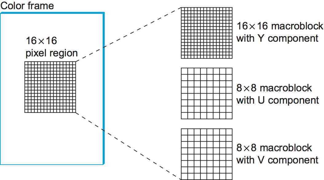
Figure 193. Each frame as a collection of macroblocks.
The P and B frames are also processed in units of macroblocks. Intuitively, we can see that the information they carry for each macroblock captures the motion in the video; that is, it shows in what direction and how far the macroblock moved relative to the reference frame(s). The following describes how a B frame is used to reconstruct a frame during decompression; P frames are handled in a similar manner, except that they depend on only one reference frame instead of two.
Before getting to the details of how a B frame is decompressed, we first note that each macroblock in a B frame is not necessarily defined relative to both an earlier and a later frame, as suggested above, but may instead simply be specified relative to just one or the other. In fact, a given macroblock in a B frame can use the same intracoding as is used in an I frame. This flexibility exists because if the motion picture is changing too rapidly then it sometimes makes sense to give the intrapicture encoding rather than a forward- or backward-predicted encoding. Thus, each macroblock in a B frame includes a type field that indicates which encoding is used for that macroblock. In the following discussion, however, we consider only the general case in which the macroblock uses bidirectional predictive encoding.
In such a case, each macroblock in a B frame is represented with a 4-tuple: (1) a coordinate for the macroblock in the frame, (2) a motion vector relative to the previous reference frame, (3) a motion vector relative to the subsequent reference frame, and (4) a delta (\(\delta\)) for each pixel in the macroblock (i.e., how much each pixel has changed relative to the two reference pixels). For each pixel in the macroblock, the first task is to find the corresponding reference pixel in the past and future reference frames. This is done using the two motion vectors associated with the macroblock. Then, the delta for the pixel is added to the average of these two reference pixels. Stated more precisely, if we let Fp and Ff denote the past and future reference frames, respectively, and the past/future motion vectors are given by (xp, yp) and (xf, yf), then the pixel at coordinate (x,y) in the current frame (denoted Fc) is computed as
where \(\delta\) is the delta for the pixel as specified in the B frame. These deltas are encoded in the same way as pixels in I frames; that is, they are run through DCT and then quantized. Since the deltas are typically small, most of the DCT coefficients are 0 after quantization; hence, they can be effectively compressed.
It should be fairly clear from the preceding discussion how encoding would be performed, with one exception. When generating a B or P frame during compression, MPEG must decide where to place the macroblocks. Recall that each macroblock in a P frame, for example, is defined relative to a macroblock in an I frame, but that the macroblock in the P frame need not be in the same part of the frame as the corresponding macroblock in the I frame—the difference in position is given by the motion vector. You would like to pick a motion vector that makes the macroblock in the P frame as similar as possible to the corresponding macroblock in the I frame, so that the deltas for that macroblock can be as small as possible. This means that you need to figure out where objects in the picture moved from one frame to the next. This is the problem of motion estimation, and several techniques (heuristics) for solving this problem are known. (We discuss papers that consider this problem at the end of this chapter.) The difficulty of this problem is one of the reasons why MPEG encoding takes longer than decoding on equivalent hardware. MPEG does not specify any particular technique; it only defines the format for encoding this information in B and P frames and the algorithm for reconstructing the pixel during decompression, as given above.
Effectiveness and Performance
MPEG typically achieves a compression ratio of 90:1, although ratios as high as 150:1 are not unheard of. In terms of the individual frame types, we can expect a compression ratio of approximately 30:1 for the I frames (this is consistent with the ratios achieved using JPEG when 24-bit color is first reduced to 8-bit color), while P and B frame compression ratios are typically three to five times smaller than the rates for the I frame. Without first reducing the 24 bits of color to 8 bits, the achievable compression with MPEG is typically between 30:1 and 50:1.
MPEG involves an expensive computation. On the compression side, it is typically done offline, which is not a problem for preparing movies for a video-on-demand service. Video can be compressed in real time using hardware today, but software implementations are quickly closing the gap. On the decompression side, low-cost MPEG video boards are available, but they do little more than YUV color lookup, which fortunately is the most expensive step. Most of the actual MPEG decoding is done in software. In recent years, processors have become fast enough to keep pace with 30-frames-per-second video rates when decoding MPEG streams purely in software—modern processors can even decode MPEG streams of high definition video (HDTV).
Video Encoding Standards
We conclude by noting that MPEG is an evolving standard of significant complexity. This complexity comes from a desire to give the encoding algorithm every possible degree of freedom in how it encodes a given video stream, resulting in different video transmission rates. It also comes from the evolution of the standard over time, with the Moving Picture Experts Group working hard to retain backwards compatibility (e.g., MPEG-1, MPEG-2, MPEG-4). What we describe in this book is the essential ideas underlying MPEG-based compression, but certainly not all the intricacies involved in an international standard.
What’s more, MPEG is not the only standard available for encoding video. For example, the ITU-T has also defined the H series for encoding real-time multimedia data. Generally, the H series includes standards for video, audio, control, and multiplexing (e.g., mixing audio, video, and data onto a single bit stream). Within the series, H.261 and H.263 were the first- and second-generation video encoding standards. In principle, both H.261 and H.263 look a lot like MPEG: They use DCT, quantization, and interframe compression. The differences between H.261/H.263 and MPEG are in the details.
Today, a partnership between the ITU-T and the MPEG group has lead to the joint H.264/MPEG-4 standard, which is used for both Blu-ray Discs and by many popular streaming sources (e.g., YouTube, Vimeo).
7.2.4 Transmitting MPEG over a Network
As we’ve noted, MPEG and JPEG are not just compression standards but also definitions of the format of video and images, respectively. Focusing on MPEG, the first thing to keep in mind is that it defines the format of a video stream; it does not specify how this stream is broken into network packets. Thus, MPEG can be used for videos stored on disk, as well as videos transmitted over a stream-oriented network connection, like that provided by TCP.
What we describe below is called the main profile of an MPEG video stream that is being sent over a network. You can think of an MPEG profile as being analogous to a “version,” except the profile is not explicitly specified in an MPEG header; the receiver has to deduce the profile from the combination of header fields it sees.
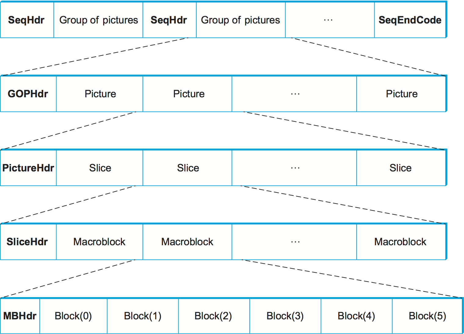
Figure 194. Format of an MPEG-compressed video stream.
A main profile MPEG stream has a nested structure, as illustrated in
Figure 194. (Keep in mind that this figure hides
a lot of messy details.) At the outermost level, the video contains
a sequence of groups of pictures (GOP) separated by a SeqHdr. The
sequence is terminated by a SeqEndCode (0xb7). The SeqHdr
that precedes every GOP specifies—among other things—the size of each
picture (frame) in the GOP (measured in both pixels and macroblocks),
the interpicture period (measured in μs), and two quantization
matrices for the macroblocks within this GOP: one for intracoded
macroblocks (I blocks) and one for intercoded macroblocks (B and
P blocks). Since this information is given for each GOP—rather than
once for the entire video stream, as you might expect—it is possible
to change the quantization table and frame rate at GOP boundaries
throughout the video. This makes it possible to adapt the video stream
over time, as we discuss below.
Each GOP is given by a GOPHdr, followed by the set of pictures that
make up the GOP. The GOPHdr specifies the number of pictures in the
GOP, as well as synchronization information for the GOP (i.e., when the
GOP should play, relative to the beginning of the video). Each picture,
in turn, is given by a PictureHdr and a set of slices that make up
the picture. (A slice is a region of the picture, such as one horizontal
line.) The PictureHdr identifies the type of the picture (I, B, or
P) and defines a picture-specific quantization table. The SliceHdr
gives the vertical position of the slice, plus another opportunity to
change the quantization table—this time by a constant scaling factor
rather than by giving a whole new table. Next, the SliceHdr is
followed by a sequence of macroblocks. Finally, each macroblock includes
a header that specifies the block address within the picture, along with
data for the six blocks within the macroblock: one for the U component,
one for the V component, and four for the Y component. (Recall that the
Y component is 16 × 16, while the U and V components are 8 × 8.)
It should be clear that one of the powers of the MPEG format is that it gives the encoder an opportunity to change the encoding over time. It can change the frame rate, the resolution, the mix of frame types that define a GOP, the quantization table, and the encoding used for individual macroblocks. As a consequence, it is possible to adapt the rate at which a video is transmitted over a network by trading picture quality for network bandwidth. Exactly how a network protocol might exploit this adaptability is currently a subject of research (see sidebar).
Another interesting aspect of sending an MPEG stream over the network is exactly how the stream is broken into packets. If sent over a TCP connection, packetization is not an issue; TCP decides when it has enough bytes to send the next IP datagram. When using video interactively, however, it is rare to transmit it over TCP, since TCP has several features that are ill suited to highly latency-sensitive applications (such as abrupt rate changes after a packet loss and retransmission of lost packets). If we are transmitting video using UDP, say, then it makes sense to break the stream at carefully selected points, such as at macroblock boundaries. This is because we would like to confine the effects of a lost packet to a single macroblock, rather than damaging several macroblocks with a single loss. This is an example of Application Level Framing, which was discussed in an earlier chapter.
Packetizing the stream is only the first problem in sending MPEG-compressed video over a network. The next complication is dealing with packet loss. On the one hand, if a B frame is dropped by the network, then it is possible to simply replay the previous frame without seriously compromising the video; 1 frame out of 30 is no big deal. On the other hand, a lost I frame has serious consequences—none of the subsequent B and P frames can be processed without it. Thus, losing an I frame would result in losing multiple frames of the video. While you could retransmit the missing I frame, the resulting delay would probably not be acceptable in a real-time videoconference. One solution to this problem would be to use the Differentiated Services techniques described in the previous chapter to mark the packets containing I frames with a lower drop probability than other packets.
One final observation is that how you choose to encode video depends on more than just the available network bandwidth. It also depends on the application’s latency constraints. Once again, an interactive application like videoconferencing needs small latencies. The critical factor is the combination of I, P, and B frames in the GOP. Consider the following GOP:
I B B B B P B B B B I
The problem this GOP causes a videoconferencing application is that the sender has to delay the transmission of the four B frames until the P or I that follows them is available. This is because each B frame depends on the subsequent P or I frame. If the video is playing at 15 frames per second (i.e., one frame every 67 ms), this means the first B frame is delayed 4 × 67 ms, which is more than a quarter of a second. This delay is in addition to any propagation delay imposed by the network. A quarter of a second is far greater than the 100-ms threshold that humans are able to perceive. It is for this reason that many videoconference applications encode video using JPEG, which is often called motion-JPEG. (Motion-JPEG also addresses the problem of dropping a reference frame since all frames are able to stand alone.) Notice, however, that an interframe encoding that depends upon only prior frames rather than later frames is not a problem. Thus, a GOP of
I P P P P I
would work just fine for interactive videoconferencing.
Adaptive Streaming
Because encoding schemes like MPEG allow for a trade-off between the bandwidth consumed and the quality of the image, there is an opportunity to adapt a video stream to match the available network bandwidth. This is effectively what video streaming services like Netflix do today.
For starters, let’s assume that we have some way to measure the amount of free capacity and level of congestion along a path, for example, by observing the rate at which packets are successfully arriving at the destination. As the available bandwidth fluctuates, we can feed that information back to the codec so that it adjusts its coding parameters to back off during congestion and to send more aggressively (with a higher picture quality) when the network is idle. This is analogous to the behavior of TCP, except in the video case we are actually modifying the total amount of data sent rather than how long we take to send a fixed amount of data, since we don’t want to introduce delay into a video application.
In the case of video-on-demand services like Netflix, we don’t adapt the encoding on the fly, but instead we encode a handful of video quality levels ahead of time, and save them to files named accordingly. The receiver simply changes the file name it requests to match the quality its measurements indicate the network will be able to deliver. The receiver watches its playback queue, and asks for a higher quality encoding when the queue becomes too full and a lower quality encoding when the queue becomes too empty.
How does this approach know where in the movie to jump to should the requested quality change? In effect, the receiver never asks the sender to stream the whole movie, but instead it requests a sequence of short movie segments, typically a few seconds long (and always on GOP boundary). Each segment is an opportunity to change the quality level to match what the network is able to deliver. (It turns out that requesting movie chunks also makes it easier to implement trick play, jumping around from one place to another in the movie.) In other words, a movie is typically stored as a set of N × M chunks (files): N quality levels for each of M segments.
There’s one last detail. Since the receiver is effectively requesting a sequence of discrete video chunks by name, the most common approach for issuing these requests is to use HTTP. Each chuck is a separate HTTP GET request with the URL identifying the specific chunk the receiver wants next. When you start downloading a movie, your video player first downloads a manifest file that contains nothing more than the URLs for the N × M chunks in the movie, and then it issues a sequence of HTTP requests using the appropriate URL for the situation. This general approach is called HTTP adaptive streaming, although it has been standardized in slightly different ways by various organizations, most notably MPEG’s DASH (Dynamic Adaptive Streaming over HTTP) and Apple’s HLS (HTTP Live Streaming).
7.2.5 Audio Compression (MP3)
Not only does MPEG define how video is compressed, but it also defines a standard for compressing audio. This standard can be used to compress the audio portion of a movie (in which case the MPEG standard defines how the compressed audio is interleaved with the compressed video in a single MPEG stream) or it can be used to compress stand-alone audio (for example, an audio CD). The MPEG audio compression standard is just one of many for audio compression, but the pivotal role it played means that MP3 (which stands for MPEG Layer III—see below) has become almost synonymous with audio compression.
To understand audio compression, we need to begin with the data. CD-quality audio, which is the de facto digital representation for high-quality audio, is sampled at a rate of 44.1 KHz (i.e., a sample is collected approximately once every 23 μs). Each sample is 16 bits, which means that a stereo (2-channel) audio stream results in a bit rate of
2 × 44.1 × 1000 × 16 = 1.41 Mbps
By comparison, traditional telephone-quality voice is sampled at a rate of 8 KHz, with 8-bit samples, resulting in a bit rate of 64 kbps.
Clearly, some amount of compression is going to be required to transmit CD-quality audio over a network of limited bandwidth. (Consider the fact that MP3 audio streaming became popular in an era when 1.5Mbps home Internet connections were a novelty). To make matters worse, synchronization and error correction overheads inflated the number of bits stored on a CD by a factor of three, so if you just read the data from the CD and sent it over the network, you would need 4.32 Mbps.
Just like video, there is lots of redundancy in audio, and compression takes advantage of this. The MPEG standards define three levels of compression, as enumerated in Table 25. Of these, Layer III, which is more widely known as MP3, was for many years the most commonly used. In recent years, higher bandwidth codecs have proliferated as streaming audio has become the dominant way many people consume music.
Coding |
Bit Rates |
Compression Factor |
|---|---|---|
Layer I |
384 kbps |
14 |
Layer II |
192 kbps |
18 |
Layer III |
128 kbps |
12 |
To achieve these compression ratios, MP3 uses techniques that are similar to those used by MPEG to compress video. First, it splits the audio stream into some number of frequency subbands, loosely analogous to the way MPEG processes the Y, U, and V components of a video stream separately. Second, each subband is broken into a sequence of blocks, which are similar to MPEG’s macroblocks except they can vary in length from 64 to 1024 samples. (The encoding algorithm can vary the block size depending on certain distortion effects that are beyond our discussion.) Finally, each block is transformed using a modified DCT algorithm, quantized, and Huffman encoded, just as for MPEG video.
The trick to MP3 is how many subbands it elects to use and how many bits it allocates to each subband, keeping in mind that it is trying to produce the highest-quality audio possible for the target bit rate. Exactly how this allocation is made is governed by psychoacoustic models that are beyond the scope of this book, but to illustrate the idea consider that it makes sense to allocate more bits to low-frequency subbands when compressing a male voice and more bits to high-frequency subbands when compressing a female voice. Operationally, MP3 dynamically changes the quantization tables used for each subband to achieve the desired effect.
Once compressed, the subbands are packaged into fixed-size frames, and a header is attached. This header includes synchronization information, as well as the bit allocation information needed by the decoder to determine how many bits are used to encode each subband. As mentioned above, these audio frames can then be interleaved with video frames to form a complete MPEG stream. One interesting side note is that, while it might work to drop B frames in the network should congestion occur, experience teaches us that it is not a good idea to drop audio frames since users are better able to tolerate bad video than bad audio.