6.4 Advanced Congestion Control
This section explores congestion control more deeply. In doing so, it is important to understand that the standard TCP’s strategy is to control congestion once it happens, as opposed to trying to avoid congestion in the first place. In fact, TCP repeatedly increases the load it imposes on the network in an effort to find the point at which congestion occurs, and then it backs off from this point. Said another way, TCP needs to create losses to find the available bandwidth of the connection. An appealing alternative is to predict when congestion is about to happen and then to reduce the rate at which hosts send data just before packets start being discarded. We call such a strategy congestion avoidance to distinguish it from congestion control, but it’s probably most accurate to think of “avoidance” as a subset of “control.”
We describe two different approaches to congestion-avoidance. The first puts a small amount of additional functionality into the router to assist the end node in the anticipation of congestion. This approach is often referred to as Active Queue Management (AQM). The second approach attempts to avoid congestion purely from the end hosts. This approach is implemented in TCP, making it variant of the congestion control mechanisms described in the previous section.
6.4.1 Active Queue Management (DECbit, RED, ECN)
The first approach requires changes to routers, which has never been the Internet’s preferred way of introducing new features, but nonetheless, has been a constant source of consternation over the last 20 years. The problem is that while it’s generally agreed that routers are in an ideal position to detect the onset of congestion—i.e., their queues start to fill up—there has not been a consensus on exactly what the best algorithm is. The following describes two of the classic mechanisms, and concludes with a brief discussion of where things stand today.
DECbit
The first mechanism was developed for use on the Digital Network Architecture (DNA), a connectionless network with a connection-oriented transport protocol. This mechanism could, therefore, also be applied to TCP and IP. As noted above, the idea here is to more evenly split the responsibility for congestion control between the routers and the end nodes. Each router monitors the load it is experiencing and explicitly notifies the end nodes when congestion is about to occur. This notification is implemented by setting a binary congestion bit in the packets that flow through the router, hence the name DECbit. The destination host then copies this congestion bit into the ACK it sends back to the source. Finally, the source adjusts its sending rate so as to avoid congestion. The following discussion describes the algorithm in more detail, starting with what happens in the router.
A single congestion bit is added to the packet header. A router sets this bit in a packet if its average queue length is greater than or equal to 1 at the time the packet arrives. This average queue length is measured over a time interval that spans the last busy+idle cycle, plus the current busy cycle. (The router is busy when it is transmitting and idle when it is not.) Figure 166 shows the queue length at a router as a function of time. Essentially, the router calculates the area under the curve and divides this value by the time interval to compute the average queue length. Using a queue length of 1 as the trigger for setting the congestion bit is a trade-off between significant queuing (and hence higher throughput) and increased idle time (and hence lower delay). In other words, a queue length of 1 seems to optimize the power function.
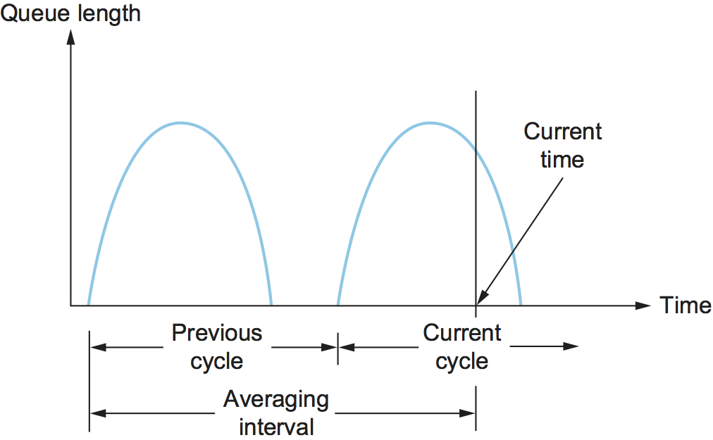
Figure 166. Computing average queue length at a router.
Now turning our attention to the host half of the mechanism, the source records how many of its packets resulted in some router setting the congestion bit. In particular, the source maintains a congestion window, just as in TCP, and watches to see what fraction of the last window’s worth of packets resulted in the bit being set. If less than 50% of the packets had the bit set, then the source increases its congestion window by one packet. If 50% or more of the last window’s worth of packets had the congestion bit set, then the source decreases its congestion window to 0.875 times the previous value. The value 50% was chosen as the threshold based on analysis that showed it to correspond to the peak of the power curve. The “increase by 1, decrease by 0.875” rule was selected because additive increase/multiplicative decrease makes the mechanism stable.
Random Early Detection
A second mechanism, called random early detection (RED), is similar to the DECbit scheme in that each router is programmed to monitor its own queue length and, when it detects that congestion is imminent, to notify the source to adjust its congestion window. RED, invented by Sally Floyd and Van Jacobson in the early 1990s, differs from the DECbit scheme in two major ways.
The first is that rather than explicitly sending a congestion notification message to the source, RED is most commonly implemented such that it implicitly notifies the source of congestion by dropping one of its packets. The source is, therefore, effectively notified by the subsequent timeout or duplicate ACK. In case you haven’t already guessed, RED is designed to be used in conjunction with TCP, which currently detects congestion by means of timeouts (or some other means of detecting packet loss such as duplicate ACKs). As the “early” part of the RED acronym suggests, the gateway drops the packet earlier than it would have to, so as to notify the source that it should decrease its congestion window sooner than it would normally have. In other words, the router drops a few packets before it has exhausted its buffer space completely, so as to cause the source to slow down, with the hope that this will mean it does not have to drop lots of packets later on.
The second difference between RED and DECbit is in the details of how RED decides when to drop a packet and what packet it decides to drop. To understand the basic idea, consider a simple FIFO queue. Rather than wait for the queue to become completely full and then be forced to drop each arriving packet (the tail drop policy of the previous section), we could decide to drop each arriving packet with some drop probability whenever the queue length exceeds some drop level. This idea is called early random drop. The RED algorithm defines the details of how to monitor the queue length and when to drop a packet.
In the following paragraphs, we describe the RED algorithm as originally proposed by Floyd and Jacobson. We note that several modifications have since been proposed both by the inventors and by other researchers. However, the key ideas are the same as those presented below, and most current implementations are close to the algorithm that follows.
First, RED computes an average queue length using a weighted running
average similar to the one used in the original TCP timeout computation.
That is, AvgLen is computed as
AvgLen = (1 - Weight) x AvgLen + Weight x SampleLen
where 0 < Weight < 1 and SampleLen is the length of the queue
when a sample measurement is made. In most software implementations, the
queue length is measured every time a new packet arrives at the gateway.
In hardware, it might be calculated at some fixed sampling interval.
The reason for using an average queue length rather than an
instantaneous one is that it more accurately captures the notion of
congestion. Because of the bursty nature of Internet traffic, queues
can become full very quickly and then become empty again. If a queue
is spending most of its time empty, then it’s probably not appropriate
to conclude that the router is congested and to tell the hosts to slow
down. Thus, the weighted running average calculation tries to detect
long-lived congestion, as indicated in the right-hand portion of
Figure 167, by filtering out short-term changes
in the queue length. You can think of the running average as a
low-pass filter, where Weight determines the time constant of the
filter. The question of how we pick this time constant is discussed
below.
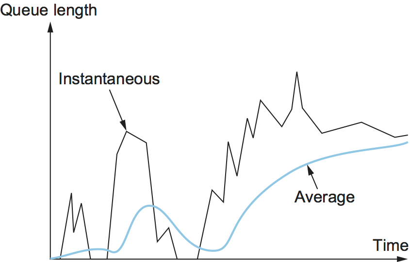
Figure 167. Weighted running average queue length.
Second, RED has two queue length thresholds that trigger certain
activity: MinThreshold and MaxThreshold. When a packet arrives
at the gateway, RED compares the current AvgLen with these two
thresholds, according to the following rules:
if AvgLen <= MinThreshold
    queue the packet
if MinThreshold < AvgLen < MaxThreshold
    calculate probability P
    drop the arriving packet with probability P
if MaxThreshold <= AvgLen
    drop the arriving packet
If the average queue length is smaller than the lower threshold, no
action is taken, and if the average queue length is larger than the
upper threshold, then the packet is always dropped. If the average
queue length is between the two thresholds, then the newly arriving
packet is dropped with some probability P. This situation is
depicted in Figure 168. The approximate
relationship between P and AvgLen is shown in Figure
169. Note that the probability of drop increases slowly
when AvgLen is between the two thresholds, reaching MaxP at
the upper threshold, at which point it jumps to unity. The rationale
behind this is that, if AvgLen reaches the upper threshold, then
the gentle approach (dropping a few packets) is not working and
drastic measures are called for: dropping all arriving packets. Some
research has suggested that a smoother transition from random dropping
to complete dropping, rather than the discontinuous approach shown
here, may be appropriate.
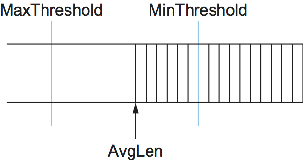
Figure 168. RED thresholds on a FIFO queue.
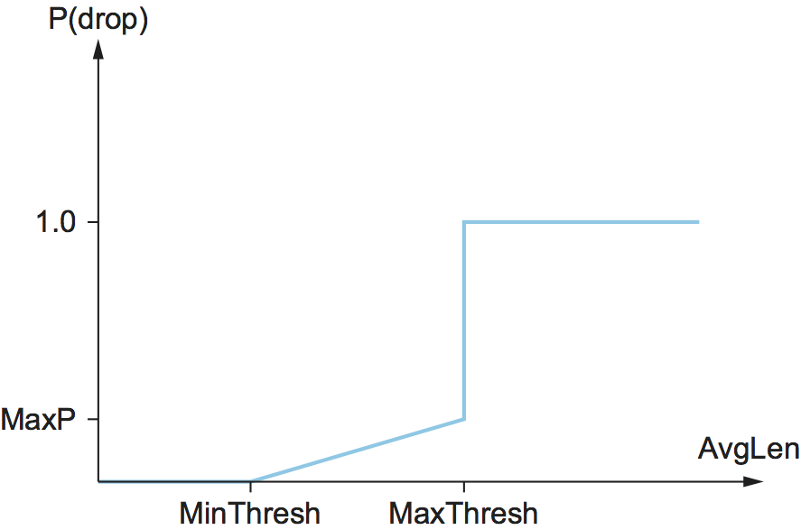
Figure 169. Drop probability function for RED.
Although Figure 169 shows the probability of
drop as a function only of AvgLen, the situation is actually a
little more complicated. In fact, P is a function of both
AvgLen and how long it has been since the last packet was
dropped. Specifically, it is computed as follows:
TempP = MaxP x (AvgLen - MinThreshold) / (MaxThreshold - MinThreshold)
P = TempP/(1 - count x TempP)
TempP is the variable that is plotted on the y-axis in Figure
169, count keeps track of how many newly arriving
packets have been queued (not dropped), and AvgLen has been between
the two thresholds. P increases slowly as count increases,
thereby making a drop increasingly likely as the time since the last
drop increases. This makes closely spaced drops relatively less likely
than widely spaced drops. This extra step in calculating P was
introduced by the inventors of RED when they observed that, without it,
the packet drops were not well distributed in time but instead tended to
occur in clusters. Because packet arrivals from a certain connection are
likely to arrive in bursts, this clustering of drops is likely to cause
multiple drops in a single connection. This is not desirable, since only
one drop per round-trip time is enough to cause a connection to reduce
its window size, whereas multiple drops might send it back into slow
start.
As an example, suppose that we set MaxP to 0.02 and count is
initialized to zero. If the average queue length were halfway between
the two thresholds, then TempP, and the initial value of P,
would be half of MaxP, or 0.01. An arriving packet, of course, has a
99 in 100 chance of getting into the queue at this point. With each
successive packet that is not dropped, P slowly increases, and by
the time 50 packets have arrived without a drop, P would have
doubled to 0.02. In the unlikely event that 99 packets arrived without
loss, P reaches 1, guaranteeing that the next packet is dropped. The
important thing about this part of the algorithm is that it ensures a
roughly even distribution of drops over time.
The intent is that, if RED drops a small percentage of packets when
AvgLen exceeds MinThreshold, this will cause a few TCP
connections to reduce their window sizes, which in turn will reduce the
rate at which packets arrive at the router. All going well, AvgLen
will then decrease and congestion is avoided. The queue length can be
kept short, while throughput remains high since few packets are dropped.
Note that, because RED is operating on a queue length averaged over
time, it is possible for the instantaneous queue length to be much
longer than AvgLen. In this case, if a packet arrives and there is
nowhere to put it, then it will have to be dropped. When this happens,
RED is operating in tail drop mode. One of the goals of RED is to
prevent tail drop behavior if possible.
The random nature of RED confers an interesting property on the algorithm. Because RED drops packets randomly, the probability that RED decides to drop a particular flow’s packet(s) is roughly proportional to the share of the bandwidth that flow is currently getting at that router. This is because a flow that is sending a relatively large number of packets is providing more candidates for random dropping. Thus, there is some sense of fair resource allocation built into RED, although it is by no means precise. While arguably fair, because RED punishes high-bandwidth flows more than low-bandwidth flows, it increases the probability of a TCP restart, which is doubly painful for those high-bandwidth flows.
Key Takeaway
Note that a fair amount of analysis has gone into setting the
various RED parameters—for example, MaxThreshold,
MinThreshold, MaxP and Weight—all in the name of
optimizing the power function (throughput-to-delay ratio). The
performance of these parameters has also been confirmed through
simulation, and the algorithm has been shown not to be overly
sensitive to them. It is important to keep in mind, however, that
all of this analysis and simulation hinges on a particular
characterization of the network workload. The real contribution of
RED is a mechanism by which the router can more accurately manage
its queue length. Defining precisely what constitutes an optimal
queue length depends on the traffic mix and is still a subject of
research, with real information now being gathered from operational
deployment of RED in the Internet. [Next]
Consider the setting of the two thresholds, MinThreshold and
MaxThreshold. If the traffic is fairly bursty, then MinThreshold
should be sufficiently large to allow the link utilization to be
maintained at an acceptably high level. Also, the difference between the
two thresholds should be larger than the typical increase in the
calculated average queue length in one RTT. Setting MaxThreshold to
twice MinThreshold seems to be a reasonable rule of thumb given the
traffic mix on today’s Internet. In addition, since we expect the
average queue length to hover between the two thresholds during periods
of high load, there should be enough free buffer space above
MaxThreshold to absorb the natural bursts that occur in Internet
traffic without forcing the router to enter tail drop mode.
We noted above that Weight determines the time constant for the
running average low-pass filter, and this gives us a clue as to how we
might pick a suitable value for it. Recall that RED is trying to send
signals to TCP flows by dropping packets during times of congestion.
Suppose that a router drops a packet from some TCP connection and then
immediately forwards some more packets from the same connection. When
those packets arrive at the receiver, it starts sending duplicate ACKs
to the sender. When the sender sees enough duplicate ACKs, it will
reduce its window size. So, from the time the router drops a packet
until the time when the same router starts to see some relief from the
affected connection in terms of a reduced window size, at least one
round-trip time must elapse for that connection. There is probably not
much point in having the router respond to congestion on time scales
much less than the round-trip time of the connections passing through
it. As noted previously, 100 ms is not a bad estimate of average
round-trip times in the Internet. Thus, Weight should be chosen such
that changes in queue length over time scales much less than 100 ms are
filtered out.
Since RED works by sending signals to TCP flows to tell them to slow down, you might wonder what would happen if those signals are ignored. This is often called the unresponsive flow problem. Unresponsive flows use more than their fair share of network resources and could cause congestive collapse if there were enough of them, just as in the days before TCP congestion control. Some of the techniques described in the next section can help with this problem by isolating certain classes of traffic from others. There is also the possibility that a variant of RED could drop more heavily from flows that are unresponsive to the initial hints that it sends.
Explicit Congestion Notification
RED is the most extensively studied AQM mechanism, but it has not been widely deployed, due in part to the fact that it does not result in ideal behavior in all circumstances. It is, however, the benchmark for understanding AQM behavior. The other thing that came out of RED is the recognition that TCP could do a better job if routers were to send a more explicit congestion signal.
That is, instead of dropping a packet and assuming TCP will eventually notice (e.g., due to the arrival of a duplicate ACK), RED (or any AQM algorithm for that matter) can do a better job if it instead marks the packet and continues to send it along its way to the destination. This idea was codified in changes to the IP and TCP headers known as Explicit Congestion Notification (ECN).
Specifically, this feedback is implemented by treating two bits in the
IP TOS field as ECN bits. One bit is set by the source to indicate
that it is ECN-capable, that is, able to react to a congestion
notification. This is called the ECT bit (ECN-Capable Transport).
The other bit is set by routers along the end-to-end path when
congestion is encountered, as computed by whatever AQM algorithm it is
running. This is called the CE bit (Congestion Encountered).
In addition to these two bits in the IP header (which are
transport-agnostic), ECN also includes the addition of two optional
flags to the TCP header. The first, ECE (ECN-Echo), communicates
from the receiver to the sender that it has received a packet with the
CE bit set. The second, CWR (Congestion Window Reduced)
communicates from the sender to the receiver that it has reduced the
congestion window.
While ECN is now the standard interpretation of two of the eight bits in
the TOS field of the IP header and support for ECN is highly
recommended, it is not required. Moreover, there is no single
recommended AQM algorithm, but instead, there is a list of requirements
a good AQM algorithm should meet. Like TCP congestion control
algorithms, every AQM algorithm has its advantages and disadvantages,
and so we need a lot of them. There is one particular scenario, however,
where the TCP congestion control algorithm and AQM algorithm are
designed to work in concert: the datacenter. We return to this use case
at the end of this section.
6.4.2 Source-Based Approaches (Vegas, BBR, DCTCP)
Unlike the previous congestion-avoidance schemes, which depended on cooperation from routers, we now describe a strategy for detecting the incipient stages of congestion—before losses occur—from the end hosts. We first give a brief overview of a collection of related mechanisms that use different information to detect the early stages of congestion, and then we describe two specific mechanisms in more detail.
The general idea of these techniques is to watch for a sign from the network that some router’s queue is building up and that congestion will happen soon if nothing is done about it. For example, the source might notice that as packet queues build up in the network’s routers, there is a measurable increase in the RTT for each successive packet it sends. One particular algorithm exploits this observation as follows: The congestion window normally increases as in TCP, but every two round-trip delays the algorithm checks to see if the current RTT is greater than the average of the minimum and maximum RTTs seen so far. If it is, then the algorithm decreases the congestion window by one-eighth.
A second algorithm does something similar. The decision as to whether or not to change the current window size is based on changes to both the RTT and the window size. The window is adjusted once every two round-trip delays based on the product
(CurrentWindow - OldWindow) x (CurrentRTT - OldRTT)
If the result is positive, the source decreases the window size by one-eighth; if the result is negative or 0, the source increases the window by one maximum packet size. Note that the window changes during every adjustment; that is, it oscillates around its optimal point.
Another change seen as the network approaches congestion is the flattening of the sending rate. A third scheme takes advantage of this fact. Every RTT, it increases the window size by one packet and compares the throughput achieved to the throughput when the window was one packet smaller. If the difference is less than one-half the throughput achieved when only one packet was in transit—as was the case at the beginning of the connection—the algorithm decreases the window by one packet. This scheme calculates the throughput by dividing the number of bytes outstanding in the network by the RTT.
TCP Vegas
The mechanism we are going to describe in more detail is similar to the last algorithm in that it looks at changes in the throughput rate or, more specifically, changes in the sending rate. However, it differs from the previous algorithm in the way it calculates throughput, and instead of looking for a change in the slope of the throughput it compares the measured throughput rate with an expected throughput rate. The algorithm, TCP Vegas, is not widely deployed in the Internet today, but the strategy it uses has been adopted by other implementations that are now being deployed.
The intuition behind the Vegas algorithm can be seen in the trace of standard TCP given in Figure 170. The top graph shown in Figure 170 traces the connection’s congestion window; it shows the same information as the traces given earlier in this section. The middle and bottom graphs depict new information: The middle graph shows the average sending rate as measured at the source, and the bottom graph shows the average queue length as measured at the bottleneck router. All three graphs are synchronized in time. In the period between 4.5 and 6.0 seconds (shaded region), the congestion window increases (top graph). We expect the observed throughput to also increase, but instead it stays flat (middle graph). This is because the throughput cannot increase beyond the available bandwidth. Beyond this point, any increase in the window size only results in packets taking up buffer space at the bottleneck router (bottom graph).
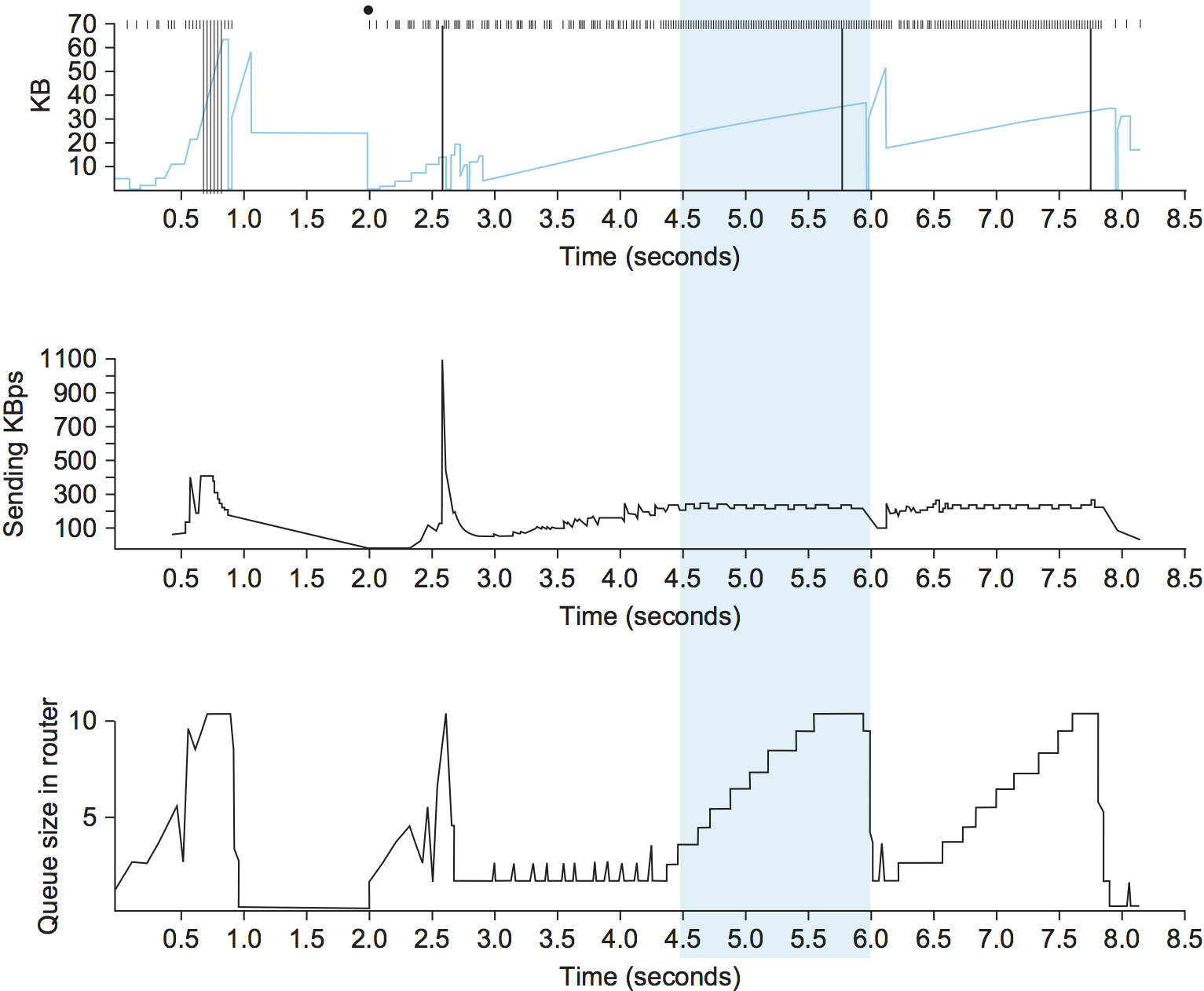
Figure 170. Congestion window versus observed throughput rate (the three graphs are synchronized). Top, congestion window; middle, observed throughput; bottom, buffer space taken up at the router. Colored line = CongestionWindow; solid bullet = timeout; hash marks = time when each packet is transmitted; vertical bars = time when a packet that was eventually retransmitted was first transmitted.
A useful metaphor that describes the phenomenon illustrated in Figure 170 is driving on ice. The speedometer (congestion window) may say that you are going 30 miles an hour, but by looking out the car window and seeing people pass you on foot (measured sending rate) you know that you are going no more than 5 miles an hour. The extra energy is being absorbed by the car’s tires (router buffers).
TCP Vegas uses this idea to measure and control the amount of extra data this connection has in transit, where by “extra data” we mean data that the source would not have transmitted had it been trying to match exactly the available bandwidth of the network. The goal of TCP Vegas is to maintain the “right” amount of extra data in the network. Obviously, if a source is sending too much extra data, it will cause long delays and possibly lead to congestion. Less obviously, if a connection is sending too little extra data, it cannot respond rapidly enough to transient increases in the available network bandwidth. TCP Vegas’s congestion-avoidance actions are based on changes in the estimated amount of extra data in the network, not only on dropped packets. We now describe the algorithm in detail.
First, define a given flow’s BaseRTT to be the RTT of a packet when
the flow is not congested. In practice, TCP Vegas sets BaseRTT to
the minimum of all measured round-trip times; it is commonly the RTT of
the first packet sent by the connection, before the router queues
increase due to traffic generated by this flow. If we assume that we are
not overflowing the connection, then the expected throughput is given by
ExpectedRate = CongestionWindow / BaseRTT
where CongestionWindow is the TCP congestion window, which we
assume (for the purpose of this discussion) to be equal to the number
of bytes in transit.
Second, TCP Vegas calculates the current sending rate, ActualRate.
This is done by recording the sending time for a distinguished packet,
recording how many bytes are transmitted between the time that packet
is sent and when its acknowledgment is received, computing the sample
RTT for the distinguished packet when its acknowledgment arrives, and
dividing the number of bytes transmitted by the sample RTT. This
calculation is done once per round-trip time.
Third, TCP Vegas compares ActualRate to ExpectedRate and
adjusts the window accordingly. We let Diff = ExpectedRate -
ActualRate. Note that Diff is positive or 0 by definition,
since ActualRate >ExpectedRate implies that we need to change
BaseRTT to the latest sampled RTT. We also define two thresholds,
α < β, roughly corresponding to having too little and too much extra
data in the network, respectively. When Diff < α, TCP Vegas
increases the congestion window linearly during the next RTT, and when
Diff > β, TCP Vegas decreases the congestion window linearly
during the next RTT. TCP Vegas leaves the congestion window unchanged
when α < Diff < β.
Intuitively, we can see that the farther away the actual throughput gets from the expected throughput, the more congestion there is in the network, which implies that the sending rate should be reduced. The β threshold triggers this decrease. On the other hand, when the actual throughput rate gets too close to the expected throughput, the connection is in danger of not utilizing the available bandwidth. The α threshold triggers this increase. The overall goal is to keep between α and β extra bytes in the network.
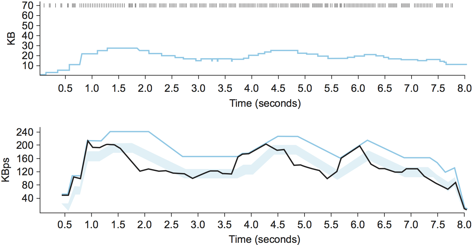
Figure 171. Trace of TCP Vegas congestion-avoidance mechanism. Top, congestion window; bottom, expected (colored line) and actual (black line) throughput. The shaded area is the region between the α and β thresholds.
Figure 171 traces the TCP Vegas
congestion-avoidance algorithm. The top graph traces the congestion
window, showing the same information as the other traces given
throughout this chapter. The bottom graph traces the expected and
actual throughput rates that govern how the congestion window is
set. It is this bottom graph that best illustrates how the algorithm
works. The colored line tracks the ExpectedRate, while the black
line tracks the ActualRate. The wide shaded strip gives the region
between the α and β thresholds; the top of the shaded strip is
α KBps away from ExpectedRate, and the bottom of the shaded
strip is β KBps away from ExpectedRate. The goal is to keep the
ActualRate between these two thresholds, within the shaded
region. Whenever ActualRate falls below the shaded region (i.e.,
gets too far from ExpectedRate), TCP Vegas decreases the
congestion window because it fears that too many packets are being
buffered in the network. Likewise, whenever ActualRate goes above
the shaded region (i.e., gets too close to the ExpectedRate), TCP
Vegas increases the congestion window because it fears that it is
underutilizing the network.
Because the algorithm, as just presented, compares the difference
between the actual and expected throughput rates to the α and β
thresholds, these two thresholds are defined in terms of KBps. However,
it is perhaps more accurate to think in terms of how many extra
buffers the connection is occupying in the network. For example, on a
connection with a BaseRTT of 100 ms and a packet size of 1 KB, if
α = 30 KBps and β = 60 KBps, then we can think of α as specifying
that the connection needs to be occupying at least 3 extra buffers in
the network and β as specifying that the connection should occupy no
more than 6 extra buffers in the network. In practice, a setting of α
to 1 buffer and β to 3 buffers works well.
Finally, you will notice that TCP Vegas decreases the congestion window linearly, seemingly in conflict with the rule that multiplicative decrease is needed to ensure stability. The explanation is that TCP Vegas does use multiplicative decrease when a timeout occurs; the linear decrease just described is an early decrease in the congestion window that should happen before congestion occurs and packets start being dropped.
TCP BBR
BBR (Bottleneck Bandwidth and RTT) is a new TCP congestion control algorithm developed by researchers at Google. Like Vegas, BBR is delay based, which means it tries to detect buffer growth so as to avoid congestion and packet loss. Both BBR and Vegas use the minimum RTT and maximum RTT, as calculated over some time interval, as their main control signals.
BBR also introduces new mechanisms to improve performance, including packet pacing, bandwidth probing, and RTT probing. Packet pacing spaces the packets based on the estimate of the available bandwidth. This eliminates bursts and unnecessary queuing, which results in a better feedback signal. BBR also periodically increases its rate, thereby probing the available bandwidth. Similarly, BBR periodically decreases its rate, thereby probing for a new minimum RTT. The RTT probing mechanism attempts to be self-synchronizing, which is to say, when there are multiple BBR flows, their respective RTT probes happen at the same time. This gives a more accurate view of the actual uncongested path RTT, which solves one of the major issues with delay-based congestion control mechanisms: having accurate knowledge of the uncongested path RTT.
BBR is actively being worked on and rapidly evolving. One major focus is fairness. For example, some experiments show CUBIC flows get 100× less bandwidth when competing with BBR flows, and other experiments show that unfairness among BBR flows is even possible. Another major focus is avoiding high retransmission rates, where in some cases as many as 10% of packets are retransmitted.
DCTCP
We conclude with an example of a situation where a variant of the TCP congestion control algorithm has been designed to work in concert with ECN: in cloud datacenters. The combination is called DCTCP, which stands for Data Center TCP. The situation is unique in that a datacenter is self-contained, and so it is possible to deploy a tailor-made version of TCP that does not need to worry about treating other TCP flows fairly. Datacenters are also unique in that they are built using commodity switches, and because there is no need to worry about long-fat pipes spanning a continent, the switches are typically provisioned without an excess of buffers.
The idea is straightforward. DCTCP adapts ECN by estimating the fraction of bytes that encounter congestion rather than simply detecting that some congestion is about to occur. At the end hosts, DCTCP then scales the congestion window based on this estimate. The standard TCP algorithm still kicks in should a packet actually be lost. The approach is designed to achieve high-burst tolerance, low latency, and high throughput with shallow-buffered switches.
The key challenge DCTCP faces is to estimate the fraction of bytes encountering congestion. Each switch is simple. If a packet arrives and the switch sees the queue length (K) is above some threshold; e.g.,
K > (RTT × C)/7
where C is the link rate in packets per second, then the switch sets the CE bit in the IP header. The complexity of RED is not required.
The receiver then maintains a boolean variable for every flow, which
we’ll denote SeenCE, and implements the following state machine in
response to every received packet:
If the CE bit is set and
SeenCE=False, setSeenCEto True and send an immediate ACK.If the CE bit is not set and
SeenCE=True, setSeenCEto False and send an immediate ACK.Otherwise, ignore the CE bit.
The non-obvious consequence of the “otherwise” case is that the receiver continues to send delayed ACKs once every n packets, whether or not the CE bit is set. This has proven important to maintaining high performance.
Finally, the sender computes the fraction of bytes that encountered congestion during the previous observation window (usually chosen to be approximately the RTT), as the ratio of the total bytes transmitted and the bytes acknowledged with the ECE flag set. DCTCP grows the congestion window in exactly the same way as the standard algorithm, but it reduces the window in proportion to how many bytes encountered congestion during the last observation window.