6.3 TCP Congestion Control
This section describes the predominant example of end-to-end congestion control in use today, that implemented by TCP. The essential strategy of TCP is to send packets into the network without a reservation and then to react to observable events that occur. TCP assumes only FIFO queuing in the network’s routers, but also works with fair queuing.
TCP congestion control was introduced into the Internet in the late 1980s by Van Jacobson, roughly eight years after the TCP/IP protocol stack had become operational. Immediately preceding this time, the Internet was suffering from congestion collapse—hosts would send their packets into the Internet as fast as the advertised window would allow, congestion would occur at some router (causing packets to be dropped), and the hosts would time out and retransmit their packets, resulting in even more congestion.
Broadly speaking, the idea of TCP congestion control is for each source to determine how much capacity is available in the network, so that it knows how many packets it can safely have in transit. Once a given source has this many packets in transit, it uses the arrival of an ACK as a signal that one of its packets has left the network and that it is therefore safe to insert a new packet into the network without adding to the level of congestion. By using ACKs to pace the transmission of packets, TCP is said to be self-clocking. Of course, determining the available capacity in the first place is no easy task. To make matters worse, because other connections come and go, the available bandwidth changes over time, meaning that any given source must be able to adjust the number of packets it has in transit. This section describes the algorithms used by TCP to address these and other problems.
Note that, although we describe the TCP congestion-control mechanisms one at a time, thereby giving the impression that we are talking about three independent mechanisms, it is only when they are taken as a whole that we have TCP congestion control. Also, while we are going to begin here with the variant of TCP congestion control most often referred to as standard TCP, we will see that there are actually quite a few variants of TCP congestion control in use today, and researchers continue to explore new approaches to addressing this problem. Some of these new approaches are discussed below.
6.3.1 Additive Increase/Multiplicative Decrease
TCP maintains a new state variable for each connection, called
CongestionWindow, which is used by the source to limit how much data
it is allowed to have in transit at a given time. The congestion window
is congestion control’s counterpart to flow control’s advertised window.
TCP is modified such that the maximum number of bytes of unacknowledged
data allowed is now the minimum of the congestion window and the
advertised window. Thus, using the variables defined in the previous
chapter, TCP’s effective window is revised as follows:
MaxWindow = MIN(CongestionWindow, AdvertisedWindow)
EffectiveWindow = MaxWindow -  (LastByteSent - LastByteAcked)
That is, MaxWindow replaces AdvertisedWindow in the calculation
of EffectiveWindow. Thus, a TCP source is allowed to send no
faster than the slowest component—the network or the destination
host—can accommodate.
The problem, of course, is how TCP comes to learn an appropriate value
for CongestionWindow. Unlike the AdvertisedWindow, which is sent
by the receiving side of the connection, there is no one to send a
suitable CongestionWindow to the sending side of TCP. The answer is
that the TCP source sets the CongestionWindow based on the level of
congestion it perceives to exist in the network. This involves
decreasing the congestion window when the level of congestion goes up
and increasing the congestion window when the level of congestion goes
down. Taken together, the mechanism is commonly called additive
increase/multiplicative decrease (AIMD); the reason for this mouthful
of a name will become apparent below.
The key question, then, is how does the source determine that the
network is congested and that it should decrease the congestion window?
The answer is based on the observation that the main reason packets are
not delivered, and a timeout results, is that a packet was dropped due
to congestion. It is rare that a packet is dropped because of an error
during transmission. Therefore, TCP interprets timeouts as a sign of
congestion and reduces the rate at which it is transmitting.
Specifically, each time a timeout occurs, the source sets
CongestionWindow to half of its previous value. This halving of the
CongestionWindow for each timeout corresponds to the “multiplicative
decrease” part of AIMD.
Although CongestionWindow is defined in terms of bytes, it is
easiest to understand multiplicative decrease if we think in terms of
whole packets. For example, suppose the CongestionWindow is
currently set to 16 packets. If a loss is detected, CongestionWindow
is set to 8. (Normally, a loss is detected when a timeout occurs, but as
we see below, TCP has another mechanism to detect dropped packets.)
Additional losses cause CongestionWindow to be reduced to 4, then 2,
and finally to 1 packet. CongestionWindow is not allowed to fall
below the size of a single packet, or in TCP terminology, the maximum
segment size .
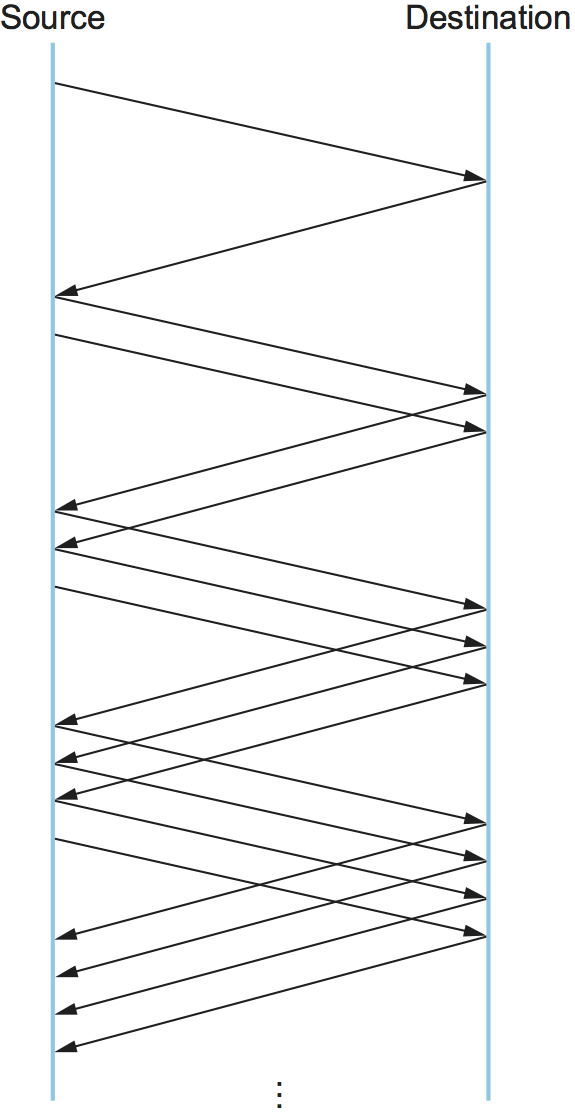
Figure 159. Packets in transit during additive increase, with one packet being added each RTT.
A congestion-control strategy that only decreases the window size is
obviously too conservative. We also need to be able to increase the
congestion window to take advantage of newly available capacity in the
network. This is the “additive increase” part of AIMD, and it works as
follows. Every time the source successfully sends a
CongestionWindow’s worth of packets—that is, each packet sent
out during the last round-trip time (RTT) has been ACKed—it adds the
equivalent of 1 packet to CongestionWindow. This linear increase
is illustrated in Figure 159. Note that, in
practice, TCP does not wait for an entire window’s worth of ACKs to
add 1 packet’s worth to the congestion window, but instead increments
CongestionWindow by a little for each ACK that
arrives. Specifically, the congestion window is incremented as follows
each time an ACK arrives:
Increment = MSS x (MSS/CongestionWindow)
CongestionWindow += Increment
That is, rather than incrementing CongestionWindow by an entire
MSS bytes each RTT, we increment it by a fraction of MSS every
time an ACK is received. Assuming that each ACK acknowledges the receipt
of MSS bytes, then that fraction is MSS/CongestionWindow.
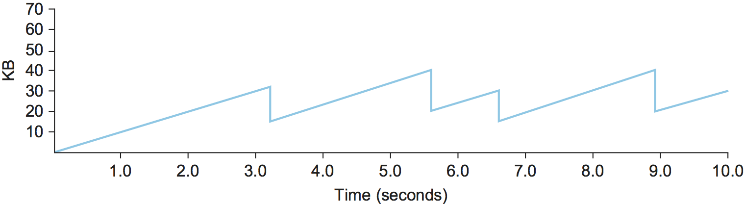
Figure 160. Typical TCP sawtooth pattern.
This pattern of continually increasing and decreasing the congestion
window continues throughout the lifetime of the connection. In fact,
if you plot the current value of CongestionWindow as a function of
time, you get a sawtooth pattern, as illustrated in Figure 160. The important concept to understand about AIMD is
that the source is willing to reduce its congestion window at a much
faster rate than it is willing to increase its congestion window. This
is in contrast to an additive increase/additive decrease strategy in
which the window would be increased by 1 packet when an ACK arrives
and decreased by 1 when a timeout occurs. It has been shown that AIMD
is a necessary condition for a congestion-control mechanism to be
stable.
An intuitive explanation for why TCP decreases the window aggressively and increases it conservatively is that the consequences of having too large a window are compounding. This is because when the window is too large, packets that are dropped will be retransmitted, making congestion even worse. It is important to get out of this state quickly.
Finally, since a timeout is an indication of congestion that triggers multiplicative decrease, TCP needs the most accurate timeout mechanism it can afford. We already covered TCP’s timeout mechanism in an earlier chapter, so we do not repeat it here. The two main things to remember about that mechanism are that (1) timeouts are set as a function of both the average RTT and the standard deviation in that average, and (2) due to the cost of measuring each transmission with an accurate clock, TCP only samples the round-trip time once per RTT (rather than once per packet) using a coarse-grained (500-ms) clock.
6.3.2 Slow Start
The additive increase mechanism just described is the right approach to use when the source is operating close to the available capacity of the network, but it takes too long to ramp up a connection when it is starting from scratch. TCP therefore provides a second mechanism, ironically called slow start, which is used to increase the congestion window rapidly from a cold start. Slow start effectively increases the congestion window exponentially, rather than linearly.
Specifically, the source starts out by setting CongestionWindow to
one packet. When the ACK for this packet arrives, TCP adds 1 to
CongestionWindow and then sends two packets. Upon receiving the
corresponding two ACKs, TCP increments CongestionWindow by 2—one
for each ACK—and next sends four packets. The end result is that TCP
effectively doubles the number of packets it has in transit every RTT.
Figure 161 shows the growth in the number
of packets in transit during slow start. Compare this to the linear
growth of additive increase illustrated in Figure 159.
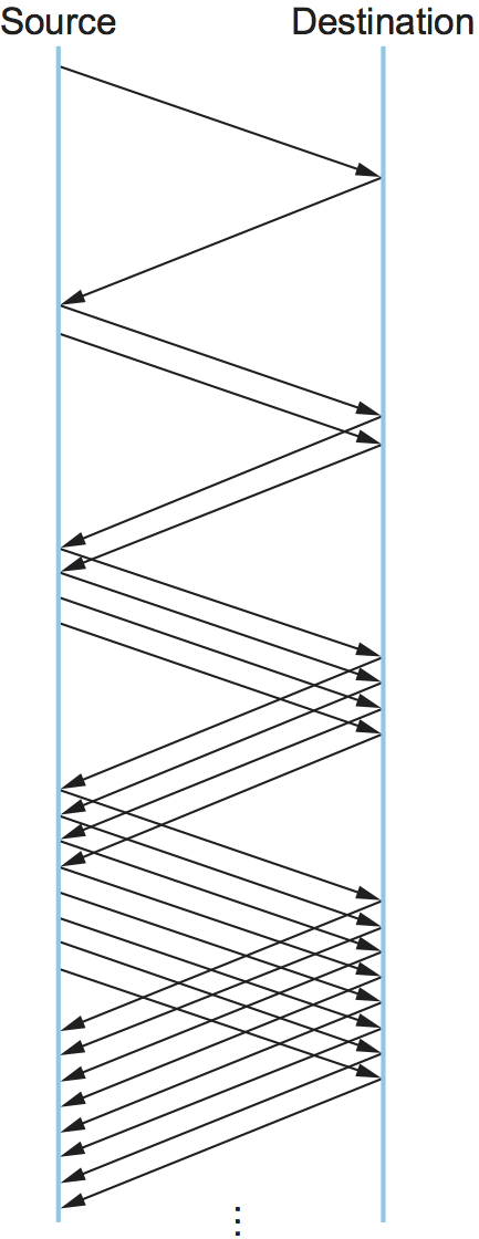
Figure 161. Packets in transit during slow start.
Why any exponential mechanism would be called “slow” is puzzling at first, but it can be explained if put in the proper historical context. We need to compare slow start not against the linear mechanism of the previous subsection, but against the original behavior of TCP. Consider what happens when a connection is established and the source first starts to send packets—that is, when it currently has no packets in transit. If the source sends as many packets as the advertised window allows—which is exactly what TCP did before slow start was developed—then even if there is a fairly large amount of bandwidth available in the network, the routers may not be able to consume this burst of packets. It all depends on how much buffer space is available at the routers. Slow start was therefore designed to space packets out so that this burst does not occur. In other words, even though its exponential growth is faster than linear growth, slow start is much “slower” than sending an entire advertised window’s worth of data all at once.
There are actually two different situations in which slow start runs.
The first is at the very beginning of a connection, at which time the
source has no idea how many packets it is going to be able to have in
transit at a given time. (Keep in mind that today TCP runs over
everything from 1-Mbps links to 40-Gbps links, so there is no way for
the source to know the network’s capacity.) In this situation, slow
start continues to double CongestionWindow each RTT until there is a
loss, at which time a timeout causes multiplicative decrease to divide
CongestionWindow by 2.
The second situation in which slow start is used is a bit more subtle; it occurs when the connection goes dead while waiting for a timeout to occur. Recall how TCP’s sliding window algorithm works—when a packet is lost, the source eventually reaches a point where it has sent as much data as the advertised window allows, and so it blocks while waiting for an ACK that will not arrive. Eventually, a timeout happens, but by this time there are no packets in transit, meaning that the source will receive no ACKs to “clock” the transmission of new packets. The source will instead receive a single cumulative ACK that reopens the entire advertised window, but, as explained above, the source then uses slow start to restart the flow of data rather than dumping a whole window’s worth of data on the network all at once.
Although the source is using slow start again, it now knows more
information than it did at the beginning of a connection. Specifically,
the source has a current (and useful) value of CongestionWindow;
this is the value of CongestionWindow that existed prior to the last
packet loss, divided by 2 as a result of the loss. We can think of this
as the target congestion window. Slow start is used to rapidly
increase the sending rate up to this value, and then additive increase
is used beyond this point. Notice that we have a small bookkeeping
problem to take care of, in that we want to remember the target
congestion window resulting from multiplicative decrease as well as the
actual congestion window being used by slow start. To address this
problem, TCP introduces a temporary variable to store the target window,
typically called CongestionThreshold, that is set equal to the
CongestionWindow value that results from multiplicative decrease.
The variable CongestionWindow is then reset to one packet, and it is
incremented by one packet for every ACK that is received until it
reaches CongestionThreshold, at which point it is incremented by one
packet per RTT.
In other words, TCP increases the congestion window as defined by the following code fragment:
{
    u_int    cw = state->CongestionWindow;
    u_int    incr = state->maxseg;

    if (cw > state->CongestionThreshold)
        incr = incr * incr / cw;
    state->CongestionWindow = MIN(cw + incr, TCP_MAXWIN);
}
where state represents the state of a particular TCP connection and
defines an upper bound on how large the congestion window is allowed to
grow.
Figure 162 traces how TCP’s CongestionWindow
increases and decreases over time and serves to illustrate the
interplay of slow start and additive increase/multiplicative
decrease. This trace was taken from an actual TCP connection and shows
the current value of CongestionWindow—the colored line—over time.
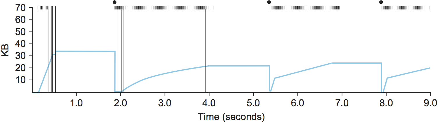
Figure 162. Behavior of TCP congestion control. Colored line = value of CongestionWindow over time; solid bullets at top of graph = timeouts; hash marks at top of graph = time when each packet is transmitted; vertical bars = time when a packet that was eventually retransmitted was first transmitted.
There are several things to notice about this trace. The first is the
rapid increase in the congestion window at the beginning of the
connection. This corresponds to the initial slow start phase. The slow
start phase continues until several packets are lost at about 0.4
seconds into the connection, at which time CongestionWindow flattens
out at about 34 KB. (Why so many packets are lost during slow start is
discussed below.) The reason why the congestion window flattens is that
there are no ACKs arriving, due to the fact that several packets were
lost. In fact, no new packets are sent during this time, as denoted by
the lack of hash marks at the top of the graph. A timeout eventually
happens at approximately 2 seconds, at which time the congestion window
is divided by 2 (i.e., cut from approximately 34 KB to around 17 KB) and
CongestionThreshold is set to this value. Slow start then causes
CongestionWindow to be reset to one packet and to start ramping up
from there.
There is not enough detail in the trace to see exactly what happens when
a couple of packets are lost just after 2 seconds, so we jump ahead to
the linear increase in the congestion window that occurs between 2 and
4 seconds. This corresponds to additive increase. At about 4 seconds,
CongestionWindow flattens out, again due to a lost packet. Now, at
about 5.5 seconds:
A timeout happens, causing the congestion window to be divided by 2, dropping it from approximately 22 KB to 11 KB, and
CongestionThresholdis set to this amount.CongestionWindowis reset to one packet, as the sender enters slow start.Slow start causes
CongestionWindowto grow exponentially until it reachesCongestionThreshold.CongestionWindowthen grows linearly.
The same pattern is repeated at around 8 seconds when another timeout occurs.
We now return to the question of why so many packets are lost during the initial slow start period. At this point, TCP is attempting to learn how much bandwidth is available on the network. This is a difficult task. If the source is not aggressive at this stage—for example, if it only increases the congestion window linearly—then it takes a long time for it to discover how much bandwidth is available. This can have a dramatic impact on the throughput achieved for this connection. On the other hand, if the source is aggressive at this stage, as TCP is during exponential growth, then the source runs the risk of having half a window’s worth of packets dropped by the network.
To see what can happen during exponential growth, consider the situation in which the source was just able to successfully send 16 packets through the network, causing it to double its congestion window to 32. Suppose, however, that the network happens to have just enough capacity to support 16 packets from this source. The likely result is that 16 of the 32 packets sent under the new congestion window will be dropped by the network; actually, this is the worst-case outcome, since some of the packets will be buffered in some router. This problem will become increasingly severe as the delay × bandwidth product of networks increases. For example, a delay × bandwidth product of 500 KB means that each connection has the potential to lose up to 500 KB of data at the beginning of each connection. Of course, this assumes that both the source and the destination implement the “big windows” extension.
Alternatives to slow start, whereby the source tries to estimate the available bandwidth by more sophisticated means, have also been explored. One example is called quick-start. The basic idea is that a TCP sender can ask for an initial sending rate greater than slow start would allow by putting a requested rate in its SYN packet as an IP option. Routers along the path can examine the option, evaluate the current level of congestion on the outgoing link for this flow, and decide if that rate is acceptable, if a lower rate would be acceptable, or if standard slow start should be used. By the time the SYN reaches the receiver, it will contain either a rate that was acceptable to all routers on the path or an indication that one or more routers on the path could not support the quick-start request. In the former case, the TCP sender uses that rate to begin transmission; in the latter case, it falls back to standard slow start. If TCP is allowed to start off sending at a higher rate, a session could more quickly reach the point of filling the pipe, rather than taking many round-trip times to do so.
Clearly one of the challenges to this sort of enhancement to TCP is that it requires substantially more cooperation from the routers than standard TCP does. If a single router in the path does not support quick-start, then the system reverts to standard slow start. Thus, it could be a long time before these types of enhancements could make it into the Internet; for now, they are more likely to be used in controlled network environments (e.g., research networks).
6.3.3 Fast Retransmit and Fast Recovery
The mechanisms described so far were part of the original proposal to add congestion control to TCP. It was soon discovered, however, that the coarse-grained implementation of TCP timeouts led to long periods of time during which the connection went dead while waiting for a timer to expire. Because of this, a new mechanism called fast retransmit was added to TCP. Fast retransmit is a heuristic that sometimes triggers the retransmission of a dropped packet sooner than the regular timeout mechanism. The fast retransmit mechanism does not replace regular timeouts; it just enhances that facility.
The idea of fast retransmit is straightforward. Every time a data packet arrives at the receiving side, the receiver responds with an acknowledgment, even if this sequence number has already been acknowledged. Thus, when a packet arrives out of order—when TCP cannot yet acknowledge the data the packet contains because earlier data has not yet arrived—TCP resends the same acknowledgment it sent the last time. This second transmission of the same acknowledgment is called a duplicate ACK. When the sending side sees a duplicate ACK, it knows that the other side must have received a packet out of order, which suggests that an earlier packet might have been lost. Since it is also possible that the earlier packet has only been delayed rather than lost, the sender waits until it sees some number of duplicate ACKs and then retransmits the missing packet. In practice, TCP waits until it has seen three duplicate ACKs before retransmitting the packet.
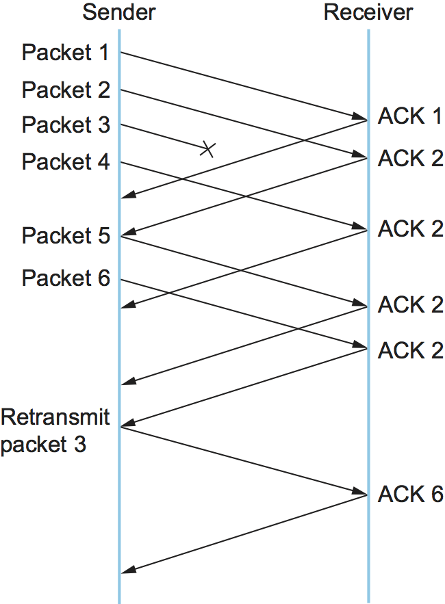
Figure 163. Fast retransmit based on duplicate ACKs.
Figure 163 illustrates how duplicate ACKs lead to a fast retransmit. In this example, the destination receives packets 1 and 2, but packet 3 is lost in the network. Thus, the destination will send a duplicate ACK for packet 2 when packet 4 arrives, again when packet 5 arrives, and so on. (To simplify this example, we think in terms of packets 1, 2, 3, and so on, rather than worrying about the sequence numbers for each byte.) When the sender sees the third duplicate ACK for packet 2—the one sent because the receiver had gotten packet 6—it retransmits packet 3. Note that when the retransmitted copy of packet 3 arrives at the destination, the receiver then sends a cumulative ACK for everything up to and including packet 6 back to the source.
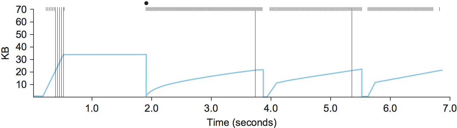
Figure 164. Trace of TCP with fast retransmit. Colored line = CongestionWindow; solid bullet = timeout; hash marks = time when each packet is transmitted; vertical bars = time when a packet that was eventually retransmitted was first transmitted.
Figure 164 illustrates the behavior of a version of TCP with the fast retransmit mechanism. It is interesting to compare this trace with that given in Figure 162, where fast retransmit was not implemented—the long periods during which the congestion window stays flat and no packets are sent has been eliminated. In general, this technique is able to eliminate about half of the coarse-grained timeouts on a typical TCP connection, resulting in roughly a 20% improvement in the throughput over what could otherwise have been achieved. Notice, however, that the fast retransmit strategy does not eliminate all coarse-grained timeouts. This is because for a small window size there will not be enough packets in transit to cause enough duplicate ACKs to be delivered. Given enough lost packets—for example, as happens during the initial slow start phase—the sliding window algorithm eventually blocks the sender until a timeout occurs. In practice, TCP’s fast retransmit mechanism can detect up to three dropped packets per window.
Finally, there is one last improvement we can make. When the fast retransmit mechanism signals congestion, rather than drop the congestion window all the way back to one packet and run slow start, it is possible to use the ACKs that are still in the pipe to clock the sending of packets. This mechanism, which is called fast recovery, effectively removes the slow start phase that happens between when fast retransmit detects a lost packet and additive increase begins. For example, fast recovery avoids the slow start period between 3.8 and 4 seconds in Figure 164 and instead simply cuts the congestion window in half (from 22 KB to 11 KB) and resumes additive increase. In other words, slow start is only used at the beginning of a connection and whenever a coarse-grained timeout occurs. At all other times, the congestion window is following a pure additive increase/multiplicative decrease pattern.
6.3.4 TCP CUBIC
A variant of the standard TCP algorithm just described, called CUBIC, is the default congestion control algorithm distributed with Linux. CUBIC’s primary goal is to support networks with large delay × bandwidth products, which are sometimes called long-fat networks. Such networks suffer from the original TCP algorithm requiring too many round-trips to reach the available capacity of the end-to-end path. CUBIC does this by being more aggressive in how it increases the window size, but of course the trick is to be more aggressive without being so aggressive as to adversely affect other flows.
One important aspect of CUBIC’s approach is to adjust its congestion window at regular intervals, based on the amount of time that has elapsed since the last congestion event (e.g., the arrival of a duplicate ACK), rather than only when ACKs arrive (the latter being a function of RTT). This allows CUBIC to behave fairly when competing with short-RTT flows, which will have ACKs arriving more frequently.
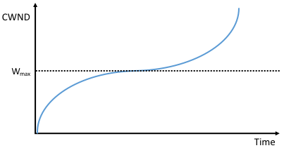
Figure 165. Generic cubic function illustrating the change in the congestion window as a function of time.
The second important aspect of CUBIC is its use of a cubic function to adjust the congestion window. The basic idea is easiest to understand by looking at the general shape of a cubic function, which has three phases: slowing growth, flatten plateau, increasing growth. A generic example is shown in Figure 165, which we have annotated with one extra piece of information: the maximum congestion window size achieved just before the last congestion event as a target (denoted \(W_{max}\)). The idea is to start fast but slow the growth rate as you get close to \(W_{max}\), be cautious and have near-zero growth when close to \(W_{max}\), and then increase the growth rate as you move away from \(W_{max}\). The latter phase is essentially probing for a new achievable \(W_{max}\).
Specifically, CUBIC computes the congestion window as a function of time (t) since the last congestion event
where
C is a scaling constant and \(\beta\) is the multiplicative decrease factor. CUBIC sets the latter to 0.7 rather than the 0.5 that standard TCP uses. Looking back at Figure 165, CUBIC is often described as shifting between a concave function to being convex (whereas standard TCP’s additive function is only convex).