2.8 Access Networks
In addition to the Ethernet and Wi-Fi connections we typically use to connect to the Internet at home, at work, at school, and in many public spaces, most of us connect to the Internet over an access or broadband service that we buy from an ISP. This section describes two such technologies: Passive Optical Networks (PON), commonly referred to as fiber-to-the-home, and Cellular Networks that connect our mobile devices. In both cases, the networks are multi-access (like Ethernet and Wi-Fi), but as we will see, their approach to mediating access is quite different.
To set a little more context, ISPs (e.g., Telco or Cable companies) often operate a national backbone, and connected to the periphery of that backbone are hundreds or thousands of edge sites, each of which serves a city or neighborhood. These edge sites are commonly called Central Offices in the Telco world and Head Ends in the cable world, but despite their names implying “centralized” and “root of the hierarchy” these sites are at the very edge of the ISP’s network; the ISP-side of the last-mile that directly connects to customers. PON and Cellular access networks are anchored in these facilities.1
- 1
DSL is the legacy, copper-based counterpart to PON. DSL links are also terminated in Telco Central Offices, but we do not describe this technology since it is being phased out.
2.8.1 Passive Optical Network
PON is the technology most commonly used to deliver fiber-based broadband to homes and businesses. PON adopts a point-to-multipoint design, which means the network is structured as a tree, with a single point starting in the ISP’s network and then fanning out to reach up to 1024 homes. PON gets its name from the fact that the splitters are passive: they forward optical signals downstream and upstream without actively storing-and-forwarding frames. In this way, they are the optical variant of repeaters used in the classic Ethernet. Framing then happens at the source in the ISP’s premises, in a device called an Optical Line Terminal (OLT), and at the end-points in individual homes, in a device called an Optical Network Unit (ONU).
Figure 52 shows an example PON, simplified to depict just one ONU and one OLT. In practice, a Central Office would include multiple OLTs connecting to thousands of customer homes. For completeness, Figure 52 also includes two other details about how the PON is connected to the ISP’s backbone (and hence, to the rest of the Internet). The Agg Switch aggregates traffic from a set of OLTs, and the BNG (Broadband Network Gateway) is a piece of Telco equipment that, among many other things, meters Internet traffic for the sake of billing. As its name implies, the BNG is effectively the gateway between the access network (everything to the left of the BNG) and the Internet (everything to the right of the BNG).
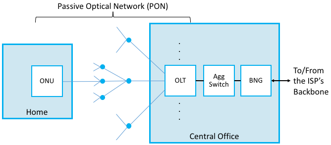
Figure 52. An example PON that connects OLTs in the Central Office to ONUs in homes and businesses.
Because the splitters are passive, PON has to implement some form of multi-access protocol. The approach it adopts can be summarized as follows. First, upstream and downstream traffic are transmitted on two different optical wavelengths, so they are completely independent of each other. Downstream traffic starts at the OLT and the signal is propagated down every link in the PON. As a consequence, every frame reaches every ONU. This device then looks at a unique identifier in the individual frames sent over the wavelength, and either keeps the frame (if the identifier is for it) or drops it (if not). Encryption is used to keep ONUs from eavesdropping on their neighbors’ traffic.
Upstream traffic is then time-division multiplexed on the upstream wavelength, with each ONU periodically getting a turn to transmit. Because the ONUs are distributed over a fairly wide area (measured in kilometers) and at different distances from the OLT, it is not practical for them to transmit based on synchronized clocks, as in SONET. Instead, the OLT transmits grants to the individual ONUs, giving them a time interval during which they can transmit. In other words, the single OLT is responsible for centrally implementing the round-robin sharing of the shared PON. This includes the possibility that the OLT can grant each ONU a different share of time, effectively implementing different levels of service.
PON is similar to Ethernet in the sense that it defines a sharing algorithm that has evolved over time to accommodate higher and higher bandwidths. G-PON (Gigabit-PON) is the most widely deployed today, supporting a bandwidth of 2.25-Gbps. XGS-PON (10 Gigabit-PON) is just now starting to be deployed.
2.8.2 Cellular Network
While cellular telephone technology had its roots in analog voice communication, data services based on cellular standards are now the norm. Like Wi-Fi, cellular networks transmit data at certain bandwidths in the radio spectrum. Unlike Wi-Fi, which permits anyone to use a channel at either 2.4 or 5 GHz (all you have to do is set up a base station, as many of us do in our homes), exclusive use of various frequency bands have been auctioned off and licensed to service providers, who in turn sell mobile access service to their subscribers.
The frequency bands that are used for cellular networks vary around the world, and are complicated by the fact that ISPs often simultaneously support both old/legacy technologies and new/next-generation technologies, each of which occupies a different frequency band. The high-level summary is that traditional cellular technologies range from 700-MHz to 2400-MHz, with new mid-spectrum allocations now happening at 6-GHz and millimeter-wave (mmWave) allocations opening above 24-GHz.
Like 802.11, cellular technology relies on the use of base stations that are connected to a wired network. In the case of the cellular network, the base stations are often called Broadband Base Units (BBU), the mobile devices that connect to them are usually referred to as User Equipment (UE), and the set of BBUs are anchored at an Evolved Packet Core (EPC) hosted in a Central Office. The wireless network served by the EPC is often called a Radio Access Network (RAN).
BBUs officially go by another name—Evolved NodeB, often abbreviated eNodeB or eNB—where NodeB is what the radio unit was called in an early incarnation of cellular networks (and has since evolved). Given that the cellular world continues to evolve at a rapid pace and eNB’s are soon to be upgraded to gNB’s, we have decided to use the more generic and less cryptic BBU.
Figure 53 depicts one possible configuration of the end-to-end scenario, with a few additional bits of detail. The EPC has multiple subcomponents, including an MME (Mobility Management Entity), an HSS (Home Subscriber Server), and an S/PGW (Session/Packet Gateway) pair; the first tracks and manages the movement of UEs throughout the RAN, the second is a database that contains subscriber-related information, and the Gateway pair processes and forwards packets between the RAN and the Internet (it forms the EPC’s user plane). We say “one possible configuration” because the cellular standards allow wide variability in how many S/PGWs a given MME is responsible for, making it possible for a single MME to manage mobility across a wide geographic area that is served by multiple Central Offices. Finally, while not explicitly spelled out in Figure 53, it is sometimes the case that the ISP’s PON network is used to connect the remote BBUs back to the Central Office.
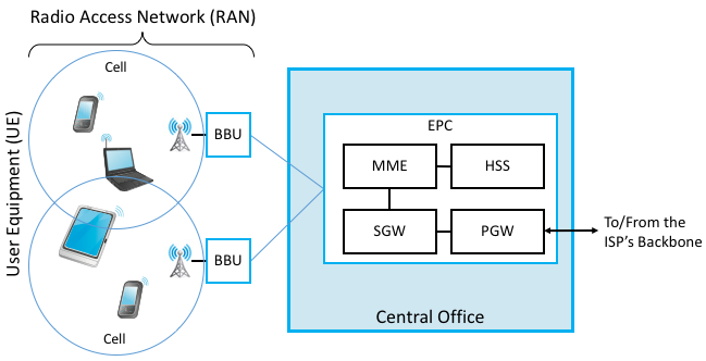
Figure 53. A Radio Access Network (RAN) connecting a set of cellular devices (UEs) to an Evolved Packet Core (EPC) hosted in a Central Office.
The geographic area served by a BBU’s antenna is called a cell. A BBU could serve a single cell or use multiple directional antennas to serve multiple cells. Cells don’t have crisp boundaries, and they overlap. Where they overlap, an UE could potentially communicate with multiple BBUs. At any time, however, the UE is in communication with, and under the control of, just one BBU. As the device begins to leave a cell, it moves into an area of overlap with one or more other cells. The current BBU senses the weakening signal from the phone and gives control of the device to whichever base station is receiving the strongest signal from it. If the device is involved in a call or other network session at the time, the session must be transferred to the new base station in what is called a handoff. The decision making process for handoffs is under the purview of the MME, which has historically been a proprietary aspect of the cellular equipment vendors (although open source MME implementations are now starting to be available).
There have been multiple generations of protocols implementing the cellular network, colloquially known as 1G, 2G, 3G, and so on. The first two generations supported only voice, with 3G defining the transition to broadband access, supporting data rates measured in hundreds of kilobits per second. Today, the industry is at 4G (supporting data rates typically measured in the few megabits per second) and is in the process of transitioning to 5G (with the promise of a tenfold increase in data rates).
As of 3G, the generational designation actually corresponds to a standard defined by the 3GPP (3rd Generation Partnership Project). Even though its name has “3G” in it, the 3GPP continues to define the standard for 4G and 5G, each of which corresponds to a release of the standard. Release 15, which is now published, is considered the demarcation point between 4G and 5G. By another name, this sequence of releases and generations is called LTE, which stands for Long-Term Evolution. The main takeaway is that while standards are published as a sequence of discrete releases, the industry as a whole has been on a fairly well-defined evolutionary path known as LTE. This section uses LTE terminology, but highlights the changes coming with 5G when appropriate.
The main innovation of LTE’s air interface is how it allocates the available radio spectrum to UEs. Unlike Wi-Fi, which is contention-based, LTE uses a reservation-based strategy. This difference is rooted in each system’s fundamental assumption about utilization: Wi-Fi assumes a lightly loaded network (and hence optimistically transmits when the wireless link is idle and backs off if contention is detected), while cellular networks assume (and strive for) high utilization (and hence explicitly assign different users to different “shares” of the available radio spectrum).
The state-of-the-art media access mechanism for LTE is called Orthogonal Frequency-Division Multiple Access (OFDMA). The idea is to multiplex data over a set of 12 orthogonal subcarrier frequencies, each of which is modulated independently. The “Multiple Access” in OFDMA implies that data can simultaneously be sent on behalf of multiple users, each on a different subcarrier frequency and for a different duration of time. The subbands are narrow (e.g., 15kHz), but the coding of user data into OFDMA symbols is designed to minimize the risk of data loss due to interference between adjacent bands.
The use of OFDMA naturally leads to conceptualizing the radio spectrum as a two-dimensional resource, as shown in Figure 54. The minimal schedulable unit, called a Resource Element (RE), corresponds to a 15kHz-wide band around one subcarrier frequency and the time it takes to transmit one OFDMA symbol. The number of bits that can be encoded in each symbol depends on the modulation rate, so for example using Quadrature Amplitude Modulation (QAM), 16-QAM yields 4 bits per symbol and 64-QAM yields 6 bits per symbol.
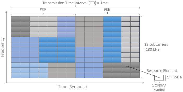
Figure 54. The available radio spectrum abstractly represented by a 2-D grid of schedulable Resource Elements.
A scheduler makes allocation decisions at the granularity of blocks of 7x12=84 resource elements, called a Physical Resource Block (PRB). Figure 54 shows two back-to-back PRBs, where UEs are depicted by different colored blocks. Of course time continues to flow along one axis, and depending on the size of the licensed frequency band, there may be many more subcarrier slots (and hence PRBs) available along the other axis, so the scheduler is essentially scheduling a sequence of PRBs for transmission.
The 1ms Transmission Time Interval (TTI) shown in Figure 54 corresponds to the time frame in which the BBU receives feedback from UEs about the quality of the signal they are experiencing. This feedback, called a Channel Quality Indicator (CQI), essentially reports the observed signal-to-noise ratio, which impacts the UE’s ability to recover the data bits. The base station then uses this information to adapt how it allocates the available radio spectrum to the UEs it is serving.
Up to this point, the description of how we schedule the radio spectrum is specific to 4G. The transition from 4G to 5G introduces additional degrees-of-freedom in how the radio spectrum is scheduled, making it possible to adapt the cellular network to a more diverse set of devices and applications domains.
Fundamentally, 5G defines a family of waveforms—unlike 4G, which specified only one waveform—each optimized for a different band in the radio spectrum.2 The bands with carrier frequencies below 1GHz are designed to deliver mobile broadband and massive IoT services with a primary focus on range. Carrier frequencies between 1GHz-6GHz are designed to offer wider bandwidths, focusing on mobile broadband and mission-critical applications. Carrier frequencies above 24GHz (mmWaves) are designed to provide super wide bandwidths over short, line-of-sight coverage.
- 2
A waveform is the frequency, amplitude, and phase-shift independent property (shape) of a signal. A sine wave is an example waveform.
These different waveforms affect the scheduling and subcarrier intervals (i.e., the “size” of the Resource Elements just described).
For sub-1GHz bands, 5G allows maximum 50MHz bandwidths. In this case, there are two waveforms: one with subcarrier spacing of 15kHz and another of 30kHz. (We used 15kHz in the example shown in Figure 54. The corresponding scheduling intervals are 0.5ms and 0.25ms, respectively. (We used 0.5ms in the example shown in Figure 54.)
For 1GHz-6GHz bands, maximum bandwidths go up to 100MHz. Correspondingly, there are three waveforms with subcarrier spacings of 15kHz, 30kHz and 60kHz, corresponding to scheduling intervals of 0.5ms, 0.25ms and 0.125ms, respectively.
For millimeter bands, bandwidths may go up to 400MHz. There are two waveforms, with subcarrier spacings of 60kHz and 120kHz. Both have scheduling intervals of 0.125ms.
This range of options is important because it adds another degree of freedom to the scheduler. In addition to allocating resource blocks to users, it has the ability to dynamically adjust the size of the resource blocks by changing the wave form being used in the band it is responsible for scheduling.
Whether 4G or 5G, the scheduling algorithm is a challenging optimization problem, with the objective of simultaneously (a) maximizing utilization of the available frequency band, and (b) ensuring that every UE receives the level of service it requires. This algorithm is not specified by 3GPP, but rather, is the proprietary intellectual property of the BBU vendors.