2.4 Error Detection
As discussed in Chapter 1, bit errors are sometimes introduced into frames. This happens, for example, because of electrical interference or thermal noise. Although errors are rare, especially on optical links, some mechanism is needed to detect these errors so that corrective action can be taken. Otherwise, the end user is left wondering why the C program that successfully compiled just a moment ago now suddenly has a syntax error in it, when all that happened in the interim is that it was copied across a network file system.
There is a long history of techniques for dealing with bit errors in computer systems, dating back to at least the 1940s. Hamming and Reed-Solomon codes are two notable examples that were developed for use in punch card readers, when storing data on magnetic disks, and in early core memories. This section describes some of the error detection techniques most commonly used in networking.
Detecting errors is only one part of the problem. The other part is correcting errors once detected. Two basic approaches can be taken when the recipient of a message detects an error. One is to notify the sender that the message was corrupted so that the sender can retransmit a copy of the message. If bit errors are rare, then in all probability the retransmitted copy will be error free. Alternatively, some types of error detection algorithms allow the recipient to reconstruct the correct message even after it has been corrupted; such algorithms rely on error-correcting codes, discussed below.
One of the most common techniques for detecting transmission errors is a technique known as the cyclic redundancy check (CRC). It is used in nearly all the link-level protocols discussed in this chapter. This section outlines the basic CRC algorithm, but before discussing that approach, we first describe the simpler checksum scheme used by several Internet protocols.
The basic idea behind any error detection scheme is to add redundant information to a frame that can be used to determine if errors have been introduced. In the extreme, we could imagine transmitting two complete copies of the data. If the two copies are identical at the receiver, then it is probably the case that both are correct. If they differ, then an error was introduced into one (or both) of them, and they must be discarded. This is a rather poor error detection scheme for two reasons. First, it sends \(n\) redundant bits for an \(n\)-bit message. Second, many errors will go undetected—any error that happens to corrupt the same bit positions in the first and second copies of the message. In general, the goal of error detecting codes is to provide a high probability of detecting errors combined with a relatively low number of redundant bits.
Fortunately, we can do a lot better than this simple scheme. In general, we can provide quite strong error detection capability while sending only \(k\) redundant bits for an \(n\)-bit message, where \(k\) is much smaller than \(n\). On an Ethernet, for example, a frame carrying up to 12,000 bits (1500 bytes) of data requires only a 32-bit CRC code, or as it is commonly expressed, uses CRC-32. Such a code will catch the overwhelming majority of errors, as we will see below.
We say that the extra bits we send are redundant because they add no new information to the message. Instead, they are derived directly from the original message using some well-defined algorithm. Both the sender and the receiver know exactly what that algorithm is. The sender applies the algorithm to the message to generate the redundant bits. It then transmits both the message and those few extra bits. When the receiver applies the same algorithm to the received message, it should (in the absence of errors) come up with the same result as the sender. It compares the result with the one sent to it by the sender. If they match, it can conclude (with high likelihood) that no errors were introduced in the message during transmission. If they do not match, it can be sure that either the message or the redundant bits were corrupted, and it must take appropriate action—that is, discarding the message or correcting it if that is possible.
One note on the terminology for these extra bits. In general, they are referred to as error-detecting codes. In specific cases, when the algorithm to create the code is based on addition, they may be called a checksum. We will see that the Internet checksum is appropriately named: It is an error check that uses a summing algorithm. Unfortunately, the word checksum is often used imprecisely to mean any form of error-detecting code, including CRCs. This can be confusing, so we urge you to use the word checksum only to apply to codes that actually do use addition and to use error-detecting code to refer to the general class of codes described in this section.
2.4.1 Internet Checksum Algorithm
Our first approach to error detection is exemplified by the Internet checksum. Although it is not used at the link level, it nevertheless provides the same sort of functionality as CRCs, so we discuss it here.
The idea behind the Internet checksum is very simple—you add up all the words that are transmitted and then transmit the result of that sum. The result is the checksum. The receiver performs the same calculation on the received data and compares the result with the received checksum. If any transmitted data, including the checksum itself, is corrupted, then the results will not match, so the receiver knows that an error occurred.
You can imagine many different variations on the basic idea of a checksum. The exact scheme used by the Internet protocols works as follows. Consider the data being checksummed as a sequence of 16-bit integers. Add them together using 16-bit ones’ complement arithmetic (explained below) and then take the ones’ complement of the result. That 16-bit number is the checksum.
In ones’ complement arithmetic, a negative integer (-x) is represented as the complement of x; that is, each bit of x is inverted. When adding numbers in ones’ complement arithmetic, a carryout from the most significant bit needs to be added to the result. Consider, for example, the addition of -5 and -3 in ones’ complement arithmetic on 4-bit integers: +5 is 0101, so -5 is 1010; +3 is 0011, so -3 is 1100. If we add 1010 and 1100, ignoring the carry, we get 0110. In ones’ complement arithmetic, the fact that this operation caused a carry from the most significant bit causes us to increment the result, giving 0111, which is the ones’ complement representation of -8 (obtained by inverting the bits in 1000), as we would expect.
The following routine gives a straightforward implementation of the
Internet’s checksum algorithm. The count argument gives the length
of buf measured in 16-bit units. The routine assumes that buf
has already been padded with 0s to a 16-bit boundary.
u_short
cksum(u_short *buf, int count)
{
    register u_long sum = 0;

    while (count--)
    {
        sum += *buf++;
        if (sum & 0xFFFF0000)
        {
            /* carry occurred, so wrap around */
            sum &= 0xFFFF;
            sum++;
        }
    }
    return ~(sum & 0xFFFF);
}
This code ensures that the calculation uses ones’ complement arithmetic
rather than the twos’ complement that is used in most machines. Note the
if statement inside the while loop. If there is a carry into the
top 16 bits of sum, then we increment sum just as in the
previous example.
Compared to our repetition code, this algorithm scores well for using a small number of redundant bits—only 16 for a message of any length—but it does not score extremely well for strength of error detection. For example, a pair of single-bit errors, one of which increments a word and one of which decrements another word by the same amount, will go undetected. The reason for using an algorithm like this in spite of its relatively weak protection against errors (compared to a CRC, for example) is simple: This algorithm is much easier to implement in software. Experience has suggested that a checksum of this form was adequate, but one reason it is adequate is that this checksum is the last line of defense in an end-to-end protocol. The majority of errors are picked up by stronger error detection algorithms, such as CRCs, at the link level.
2.4.2 Cyclic Redundancy Check
It should be clear by now that a major goal in designing error detection algorithms is to maximize the probability of detecting errors using only a small number of redundant bits. Cyclic redundancy checks use some fairly powerful mathematics to achieve this goal. For example, a 32-bit CRC gives strong protection against common bit errors in messages that are thousands of bytes long. The theoretical foundation of the cyclic redundancy check is rooted in a branch of mathematics called finite fields. While this may sound daunting, the basic ideas can be easily understood.
To start, think of an (n+1)-bit message as being represented by an \(n\) degree polynomial, that is, a polynomial whose highest-order term is \(x^{n}\). The message is represented by a polynomial by using the value of each bit in the message as the coefficient for each term in the polynomial, starting with the most significant bit to represent the highest-order term. For example, an 8-bit message consisting of the bits 10011010 corresponds to the polynomial
We can thus think of a sender and a receiver as exchanging polynomials with each other.
For the purposes of calculating a CRC, a sender and receiver have to agree on a divisor polynomial, \(C(x)\). \(C(x)\) is a polynomial of degree \(k\). For example, suppose \(C(x) = x^3 + x^2 + 1\). In this case, \(k=3\). The answer to the question “Where did \(C(x)\) come from?” is, in most practical cases, “You look it up in a book.” In fact, the choice of \(C(x)\) has a significant impact on what types of errors can be reliably detected, as we discuss below. There are a handful of divisor polynomials that are very good choices for various environments, and the exact choice is normally made as part of the protocol design. For example, the Ethernet standard uses a well-known polynomial of degree 32.
When a sender wishes to transmit a message \(M(x)\) that is n+1 bits long, what is actually sent is the (n+1)-bit message plus \(k\) bits. We call the complete transmitted message, including the redundant bits, \(P(x)\). What we are going to do is contrive to make the polynomial representing \(P(x)\) exactly divisible by \(C(x)\); we explain how this is achieved below. If \(P(x)\) is transmitted over a link and there are no errors introduced during transmission, then the receiver should be able to divide \(P(x)\) by \(C(x)\) exactly, leaving a remainder of zero. On the other hand, if some error is introduced into \(P(x)\) during transmission, then in all likelihood the received polynomial will no longer be exactly divisible by \(C(x)\), and thus the receiver will obtain a nonzero remainder implying that an error has occurred.
It will help to understand the following if you know a little about polynomial arithmetic; it is just slightly different from normal integer arithmetic. We are dealing with a special class of polynomial arithmetic here, where coefficients may be only one or zero, and operations on the coefficients are performed using modulo 2 arithmetic. This is referred to as “polynomial arithmetic modulo 2.” Since this is a networking book, not a mathematics text, let’s focus on the key properties of this type of arithmetic for our purposes (which we ask you to accept on faith):
Any polynomial \(B(x)\) can be divided by a divisor polynomial \(C(x)\) if \(B(x)\) is of higher degree than \(C(x)\).
Any polynomial \(B(x)\) can be divided once by a divisor polynomial \(C(x)\) if \(B(x)\) is of the same degree as \(C(x)\).
The remainder obtained when \(B(x)\) is divided by \(C(x)\) is obtained by performing the exclusive OR (XOR) operation on each pair of matching coefficients.
For example, the polynomial \(x^3 + 1\) can be divided by \(x^3 + x^2 + 1\) (because they are both of degree 3) and the remainder would be \(0 \times x^3 + 1 \times x^2 + 0 \times x^1 + 0 \times x^0 = x^2\) (obtained by XORing the coefficients of each term). In terms of messages, we could say that 1001 can be divided by 1101 and leaves a remainder of 0100. You should be able to see that the remainder is just the bitwise exclusive OR of the two messages.
Now that we know the basic rules for dividing polynomials, we are able to do long division, which is necessary to deal with longer messages. An example appears below.
Recall that we wanted to create a polynomial for transmission that is derived from the original message \(M(x)\), is \(k\) bits longer than \(M(x)\), and is exactly divisible by \(C(x)\). We can do this in the following way:
Multiply \(M(x)\) by \(x^{k}\); that is, add \(k\) zeros at the end of the message. Call this zero-extended message \(T(x)\).
Divide \(T(x)\) by \(C(x)\) and find the remainder.
Subtract the remainder from \(T(x)\).
It should be obvious that what is left at this point is a message that is exactly divisible by \(C(x)\). We may also note that the resulting message consists of \(M(x)\) followed by the remainder obtained in step 2, because when we subtracted the remainder (which can be no more than \(k\) bits long), we were just XORing it with the \(k\) zeros added in step 1. This part will become clearer with an example.
Consider the message \(x^7 + x^4 + x^3 + x^1\), or 10011010. We begin by multiplying by \(x^3\), since our divisor polynomial is of degree 3. This gives 10011010000. We divide this by \(C(x)\), which corresponds to 1101 in this case. Figure 32 shows the polynomial long-division operation. Given the rules of polynomial arithmetic described above, the long-division operation proceeds much as it would if we were dividing integers. Thus, in the first step of our example, we see that the divisor 1101 divides once into the first four bits of the message (1001), since they are of the same degree, and leaves a remainder of 100 (1101 XOR 1001). The next step is to bring down a digit from the message polynomial until we get another polynomial with the same degree as \(C(x)\), in this case 1001. We calculate the remainder again (100) and continue until the calculation is complete. Note that the “result” of the long division, which appears at the top of the calculation, is not really of much interest—it is the remainder at the end that matters.
You can see from the very bottom of Figure 32 that the remainder of the example calculation is 101. So we know that 10011010000 minus 101 would be exactly divisible by \(C(x)\), and this is what we send. The minus operation in polynomial arithmetic is the logical XOR operation, so we actually send 10011010101. As noted above, this turns out to be just the original message with the remainder from the long division calculation appended to it. The recipient divides the received polynomial by \(C(x)\) and, if the result is 0, concludes that there were no errors. If the result is nonzero, it may be necessary to discard the corrupted message; with some codes, it may be possible to correct a small error (e.g., if the error affected only one bit). A code that enables error correction is called an error-correcting code (ECC).
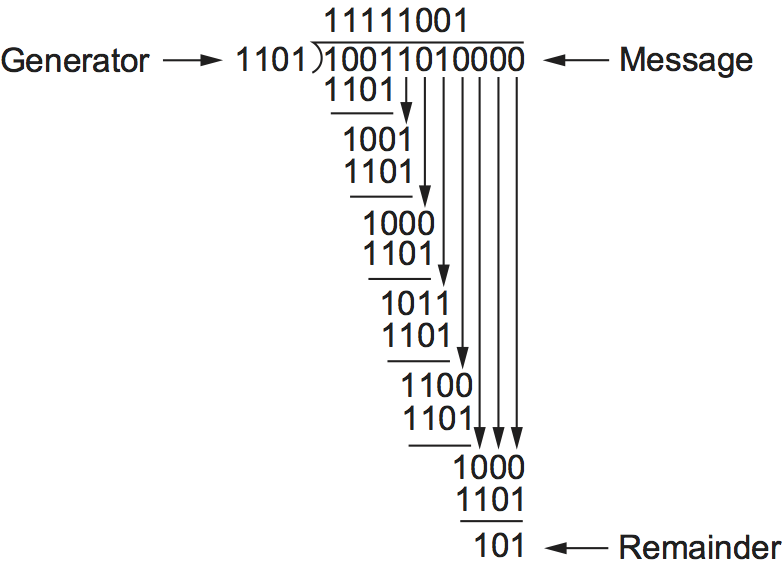
Figure 32. CRC calculation using polynomial long division.
Now we will consider the question of where the polynomial \(C(x)\) comes from. Intuitively, the idea is to select this polynomial so that it is very unlikely to divide evenly into a message that has errors introduced into it. If the transmitted message is \(P(x)\), we may think of the introduction of errors as the addition of another polynomial \(E(x)\), so the recipient sees \(P(x) + E(x)\). The only way that an error could slip by undetected would be if the received message could be evenly divided by \(C(x)\), and since we know that \(P(x)\) can be evenly divided by \(C(x)\), this could only happen if \(E(x)\) can be divided evenly by \(C(x)\). The trick is to pick \(C(x)\) so that this is very unlikely for common types of errors.
One common type of error is a single-bit error, which can be expressed as \(E(x) = x^i\) when it affects bit position i. If we select \(C(x)\) such that the first and the last term (that is, the \(x^k\) and \(x^0\) terms) are nonzero, then we already have a two-term polynomial that cannot divide evenly into the one term \(E(x)\). Such a \(C(x)\) can, therefore, detect all single-bit errors. In general, it is possible to prove that the following types of errors can be detected by a \(C(x)\) with the stated properties:
All single-bit errors, as long as the \(x^{k}\) and \(x^{0}\) terms have nonzero coefficients
All double-bit errors, as long as \(C(x)\) has a factor with at least three terms
Any odd number of errors, as long as \(C(x)\) contains the factor \((x + 1)\)
Any “burst” error (i.e., sequence of consecutive errored bits) for which the length of the burst is less than \(k\) bits (Most burst errors of length greater than \(k\) bits can also be detected.)
Six versions of \(C(x)\) are widely used in link-level protocols. For example, Ethernet uses CRC-32, which is defined as follows:
CRC-32 = \(x^{32} + x^{26} + x^{23} + x^{22} + x^{16} + x^{12} + x^{11} + x^{10} + x^8 + x^7 + x^5 + x^4 + x^2 + x + 1\)
We have mentioned that it is possible to use codes that not only detect the presence of errors but also enable errors to be corrected. Since the details of such codes require yet more complex mathematics than that required to understand CRCs, we will not dwell on them here. However, it is worth considering the merits of correction versus detection.
At first glance, it would seem that correction is always better, since with detection we are forced to throw away the message and, in general, ask for another copy to be transmitted. This uses up bandwidth and may introduce latency while waiting for the retransmission. However, there is a downside to correction, as it generally requires a greater number of redundant bits to send an error-correcting code that is as strong (that is, able to cope with the same range of errors) as a code that only detects errors. Thus, while error detection requires more bits to be sent when errors occur, error correction requires more bits to be sent all the time. As a result, error correction tends to be most useful when (1) errors are quite probable, as they may be, for example, in a wireless environment, or (2) the cost of retransmission is too high, for example, because of the latency involved retransmitting a packet over a satellite link.
The use of error-correcting codes in networking is sometimes referred to as forward error correction (FEC) because the correction of errors is handled “in advance” by sending extra information, rather than waiting for errors to happen and dealing with them later by retransmission. FEC is commonly used in wireless networks such as 802.11.
Finally, we note that the CRC algorithm, while seemingly complex, is easily implemented in hardware using a \(k\)-bit shift register and XOR gates. The number of bits in the shift register equals the degree of the generator polynomial (\(k\)). Figure 33 shows the hardware that would be used for the generator \(x^3 + x^2 + 1\) from our previous example. The message is shifted in from the left, beginning with the most significant bit and ending with the string of \(k\) zeros that is attached to the message, just as in the long division example. When all the bits have been shifted in and appropriately XORed, the register contains the remainder—that is, the CRC (most significant bit on the right). The position of the XOR gates is determined as follows: If the bits in the shift register are labeled 0 through \(k-1\), left to right, then put an XOR gate in front of bit \(n\) if there is a term \(x^n\) in the generator polynomial. Thus, we see an XOR gate in front of positions 0 and 2 for the generator \(x^3 + x^2 + x^0\).
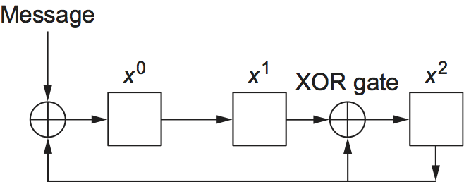
Figure 33. CRC calculation using shift register.