5.2 Reliable Byte Stream (TCP)
In contrast to a simple demultiplexing protocol like UDP, a more sophisticated transport protocol is one that offers a reliable, connection-oriented, byte-stream service. Such a service has proven useful to a wide assortment of applications because it frees the application from having to worry about missing or reordered data. The Internet’s Transmission Control Protocol is probably the most widely used protocol of this type; it is also the most carefully tuned. It is for these two reasons that this section studies TCP in detail, although we identify and discuss alternative design choices at the end of the section.
In terms of the properties of transport protocols given in the problem statement at the start of this chapter, TCP guarantees the reliable, in-order delivery of a stream of bytes. It is a full-duplex protocol, meaning that each TCP connection supports a pair of byte streams, one flowing in each direction. It also includes a flow-control mechanism for each of these byte streams that allows the receiver to limit how much data the sender can transmit at a given time. Finally, like UDP, TCP supports a demultiplexing mechanism that allows multiple application programs on any given host to simultaneously carry on a conversation with their peers.
In addition to the above features, TCP also implements a highly tuned congestion-control mechanism. The idea of this mechanism is to throttle how fast TCP sends data, not for the sake of keeping the sender from over-running the receiver, but so as to keep the sender from overloading the network. A description of TCP’s congestion-control mechanism is postponed until the next chapter, where we discuss it in the larger context of how network resources are fairly allocated.
Since many people confuse congestion control and flow control, we restate the difference. Flow control involves preventing senders from over-running the capacity of receivers. Congestion control involves preventing too much data from being injected into the network, thereby causing switches or links to become overloaded. Thus, flow control is an end-to-end issue, while congestion control is concerned with how hosts and networks interact.
5.2.1 End-to-End Issues
At the heart of TCP is the sliding window algorithm. Even though this is the same basic algorithm as is often used at the link level, because TCP runs over the Internet rather than a physical point-to-point link, there are many important differences. This subsection identifies these differences and explains how they complicate TCP. The following subsections then describe how TCP addresses these and other complications.
First, whereas the link-level sliding window algorithm presented runs over a single physical link that always connects the same two computers, TCP supports logical connections between processes that are running on any two computers in the Internet. This means that TCP needs an explicit connection establishment phase during which the two sides of the connection agree to exchange data with each other. This difference is analogous to having to dial up the other party, rather than having a dedicated phone line. TCP also has an explicit connection teardown phase. One of the things that happens during connection establishment is that the two parties establish some shared state to enable the sliding window algorithm to begin. Connection teardown is needed so each host knows it is OK to free this state.
Second, whereas a single physical link that always connects the same two computers has a fixed round-trip time (RTT), TCP connections are likely to have widely different round-trip times. For example, a TCP connection between a host in San Francisco and a host in Boston, which are separated by several thousand kilometers, might have an RTT of 100 ms, while a TCP connection between two hosts in the same room, only a few meters apart, might have an RTT of only 1 ms. The same TCP protocol must be able to support both of these connections. To make matters worse, the TCP connection between hosts in San Francisco and Boston might have an RTT of 100 ms at 3 a.m., but an RTT of 500 ms at 3 p.m. Variations in the RTT are even possible during a single TCP connection that lasts only a few minutes. What this means to the sliding window algorithm is that the timeout mechanism that triggers retransmissions must be adaptive. (Certainly, the timeout for a point-to-point link must be a settable parameter, but it is not necessary to adapt this timer for a particular pair of nodes.)
A third difference is that packets may be reordered as they cross the
Internet, but this is not possible on a point-to-point link where the
first packet put into one end of the link must be the first to appear at
the other end. Packets that are slightly out of order do not cause a
problem since the sliding window algorithm can reorder packets correctly
using the sequence number. The real issue is how far out of order
packets can get or, said another way, how late a packet can arrive at
the destination. In the worst case, a packet can be delayed in the
Internet until the IP time to live (TTL) field expires, at which
time the packet is discarded (and hence there is no danger of it
arriving late). Knowing that IP throws packets away after their TTL
expires, TCP assumes that each packet has a maximum lifetime. The exact
lifetime, known as the maximum segment lifetime (MSL), is an
engineering choice. The current recommended setting is 120 seconds. Keep
in mind that IP does not directly enforce this 120-second value; it is
simply a conservative estimate that TCP makes of how long a packet might
live in the Internet. The implication is significant—TCP has to be
prepared for very old packets to suddenly show up at the receiver,
potentially confusing the sliding window algorithm.
Fourth, the computers connected to a point-to-point link are generally engineered to support the link. For example, if a link’s delay × bandwidth product is computed to be 8 KB—meaning that a window size is selected to allow up to 8 KB of data to be unacknowledged at a given time—then it is likely that the computers at either end of the link have the ability to buffer up to 8 KB of data. Designing the system otherwise would be silly. On the other hand, almost any kind of computer can be connected to the Internet, making the amount of resources dedicated to any one TCP connection highly variable, especially considering that any one host can potentially support hundreds of TCP connections at the same time. This means that TCP must include a mechanism that each side uses to “learn” what resources (e.g., how much buffer space) the other side is able to apply to the connection. This is the flow control issue.
Fifth, because the transmitting side of a directly connected link cannot send any faster than the bandwidth of the link allows, and only one host is pumping data into the link, it is not possible to unknowingly congest the link. Said another way, the load on the link is visible in the form of a queue of packets at the sender. In contrast, the sending side of a TCP connection has no idea what links will be traversed to reach the destination. For example, the sending machine might be directly connected to a relatively fast Ethernet—and capable of sending data at a rate of 10 Gbps—but somewhere out in the middle of the network, a 1.5-Mbps link must be traversed. And, to make matters worse, data being generated by many different sources might be trying to traverse this same slow link. This leads to the problem of network congestion. Discussion of this topic is delayed until the next chapter.
We conclude this discussion of end-to-end issues by comparing TCP’s approach to providing a reliable/ordered delivery service with the approach used by virtual-circuit-based networks like the historically important X.25 network. In TCP, the underlying IP network is assumed to be unreliable and to deliver messages out of order; TCP uses the sliding window algorithm on an end-to-end basis to provide reliable/ordered delivery. In contrast, X.25 networks use the sliding window protocol within the network, on a hop-by-hop basis. The assumption behind this approach is that if messages are delivered reliably and in order between each pair of nodes along the path between the source host and the destination host, then the end-to-end service also guarantees reliable/ordered delivery.
The problem with this latter approach is that a sequence of hop-by-hop guarantees does not necessarily add up to an end-to-end guarantee. First, if a heterogeneous link (say, an Ethernet) is added to one end of the path, then there is no guarantee that this hop will preserve the same service as the other hops. Second, just because the sliding window protocol guarantees that messages are delivered correctly from node A to node B, and then from node B to node C, it does not guarantee that node B behaves perfectly. For example, network nodes have been known to introduce errors into messages while transferring them from an input buffer to an output buffer. They have also been known to accidentally reorder messages. As a consequence of these small windows of vulnerability, it is still necessary to provide true end-to-end checks to guarantee reliable/ordered service, even though the lower levels of the system also implement that functionality.
Key Takeaway
This discussion serves to illustrate one of the most important principles in system design—the end-to-end argument. In a nutshell, the end-to-end argument says that a function (in our example, providing reliable/ordered delivery) should not be provided in the lower levels of the system unless it can be completely and correctly implemented at that level. Therefore, this rule argues in favor of the TCP/IP approach. This rule is not absolute, however. It does allow for functions to be incompletely provided at a low level as a performance optimization. This is why it is perfectly consistent with the end-to-end argument to perform error detection (e.g., CRC) on a hop-by-hop basis; detecting and retransmitting a single corrupt packet across one hop is preferable to having to retransmit an entire file end-to-end. [Next]
5.2.2 Segment Format
TCP is a byte-oriented protocol, which means that the sender writes bytes into a TCP connection and the receiver reads bytes out of the TCP connection. Although “byte stream” describes the service TCP offers to application processes, TCP does not, itself, transmit individual bytes over the Internet. Instead, TCP on the source host buffers enough bytes from the sending process to fill a reasonably sized packet and then sends this packet to its peer on the destination host. TCP on the destination host then empties the contents of the packet into a receive buffer, and the receiving process reads from this buffer at its leisure. This situation is illustrated in Figure 127, which, for simplicity, shows data flowing in only one direction. Remember that, in general, a single TCP connection supports byte streams flowing in both directions.
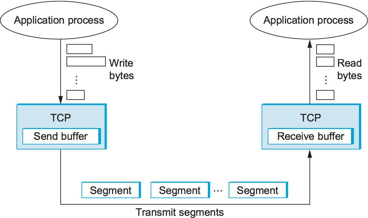
Figure 127. How TCP manages a byte stream.
The packets exchanged between TCP peers in Figure 127 are called segments, since each one carries a segment of the byte stream. Each TCP segment contains the header schematically depicted in Figure 128. The relevance of most of these fields will become apparent throughout this section. For now, we simply introduce them.
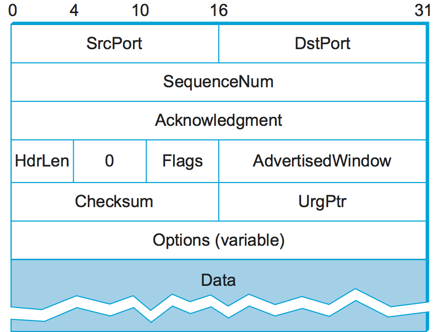
Figure 128. TCP header format.
The SrcPort and DstPort fields identify the source and
destination ports, respectively, just as in UDP. These two fields, plus
the source and destination IP addresses, combine to uniquely identify
each TCP connection. That is, TCP’s demux key is given by the 4-tuple
(SrcPort, SrcIPAddr, DstPort, DstIPAddr)
Note that because TCP connections come and go, it is possible for a connection between a particular pair of ports to be established, used to send and receive data, and closed, and then at a later time for the same pair of ports to be involved in a second connection. We sometimes refer to this situation as two different incarnations of the same connection.
The Acknowledgement, SequenceNum, and AdvertisedWindow
fields are all involved in TCP’s sliding window algorithm. Because TCP
is a byte-oriented protocol, each byte of data has a sequence number.
The SequenceNum field contains the sequence number for the first
byte of data carried in that segment, and the Acknowledgement and
AdvertisedWindow fields carry information about the flow of data
going in the other direction. To simplify our discussion, we ignore
the fact that data can flow in both directions, and we concentrate on
data that has a particular SequenceNum flowing in one direction
and Acknowledgement and AdvertisedWindow values flowing in the
opposite direction, as illustrated in Figure 129. The use of these three fields is described more fully
later in this chapter.
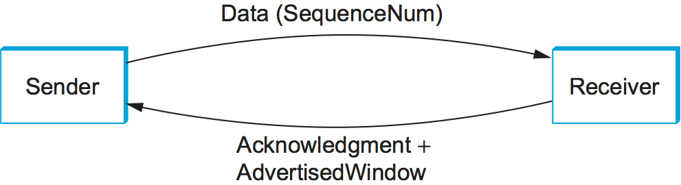
Figure 129. Simplified illustration (showing only one direction) of the TCP process, with data flow in one direction and ACKs in the other.
The 6-bit Flags field is used to relay control information between
TCP peers. The possible flags include SYN, FIN, RESET,
PUSH, URG, and ACK. The SYN and FIN flags are used
when establishing and terminating a TCP connection, respectively. Their
use is described in a later section. The ACK flag is set any time
the Acknowledgement field is valid, implying that the receiver
should pay attention to it. The URG flag signifies that this segment
contains urgent data. When this flag is set, the UrgPtr field
indicates where the nonurgent data contained in this segment begins. The
urgent data is contained at the front of the segment body, up to and
including a value of UrgPtr bytes into the segment. The PUSH
flag signifies that the sender invoked the push operation, which
indicates to the receiving side of TCP that it should notify the
receiving process of this fact. We discuss these last two features more
in a later section. Finally, the RESET flag signifies that the
receiver has become confused—for example, because it received a segment
it did not expect to receive—and so wants to abort the connection.
Finally, the Checksum field is used in exactly the same way as for
UDP—it is computed over the TCP header, the TCP data, and the
pseudoheader, which is made up of the source address, destination
address, and length fields from the IP header. The checksum is required
for TCP in both IPv4 and IPv6. Also, since the TCP header is of variable
length (options can be attached after the mandatory fields), a
HdrLen field is included that gives the length of the header in
32-bit words. This field is also known as the Offset field, since it
measures the offset from the start of the packet to the start of the
data.
5.2.3 Connection Establishment and Termination
A TCP connection begins with a client (caller) doing an active open to a server (callee). Assuming that the server had earlier done a passive open, the two sides engage in an exchange of messages to establish the connection. (Recall from Chapter 1 that a party wanting to initiate a connection performs an active open, while a party willing to accept a connection does a passive open.1) Only after this connection establishment phase is over do the two sides begin sending data. Likewise, as soon as a participant is done sending data, it closes one direction of the connection, which causes TCP to initiate a round of connection termination messages. Notice that, while connection setup is an asymmetric activity (one side does a passive open and the other side does an active open), connection teardown is symmetric (each side has to close the connection independently). Therefore, it is possible for one side to have done a close, meaning that it can no longer send data, but for the other side to keep the other half of the bidirectional connection open and to continue sending data.
- 1
To be more precise, TCP allows connection setup to be symmetric, with both sides trying to open the connection at the same time, but the common case is for one side to do an active open and the other side to do a passive open.
Three-Way Handshake
The algorithm used by TCP to establish and terminate a connection is called a three-way handshake. We first describe the basic algorithm and then show how it is used by TCP. The three-way handshake involves the exchange of three messages between the client and the server, as illustrated by the timeline given in Figure 130.
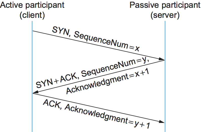
Figure 130. Timeline for three-way handshake algorithm.
The idea is that two parties want to agree on a set of parameters,
which, in the case of opening a TCP connection, are the starting
sequence numbers the two sides plan to use for their respective byte
streams. In general, the parameters might be any facts that each side
wants the other to know about. First, the client (the active
participant) sends a segment to the server (the passive participant)
stating the initial sequence number it plans to use (Flags =
SYN, SequenceNum = x). The server then responds with a single
segment that both acknowledges the client’s sequence number (Flags =
ACK, Ack = x + 1) and states its own beginning sequence number
(Flags = SYN, SequenceNum = y). That is, both the SYN and
ACK bits are set in the Flags field of this second message.
Finally, the client responds with a third segment that acknowledges
the server’s sequence number (Flags = ACK, Ack = y + 1). The
reason why each side acknowledges a sequence number that is one larger
than the one sent is that the Acknowledgement field actually
identifies the “next sequence number expected,” thereby implicitly
acknowledging all earlier sequence numbers. Although not shown in this
timeline, a timer is scheduled for each of the first two segments, and
if the expected response is not received the segment is retransmitted.
You may be asking yourself why the client and server have to exchange starting sequence numbers with each other at connection setup time. It would be simpler if each side simply started at some “well-known” sequence number, such as 0. In fact, the TCP specification requires that each side of a connection select an initial starting sequence number at random. The reason for this is to protect against two incarnations of the same connection reusing the same sequence numbers too soon—that is, while there is still a chance that a segment from an earlier incarnation of a connection might interfere with a later incarnation of the connection.
State-Transition Diagram
TCP is complex enough that its specification includes a state-transition diagram. A copy of this diagram is given in Figure 131. This diagram shows only the states involved in opening a connection (everything above ESTABLISHED) and in closing a connection (everything below ESTABLISHED). Everything that goes on while a connection is open—that is, the operation of the sliding window algorithm—is hidden in the ESTABLISHED state.
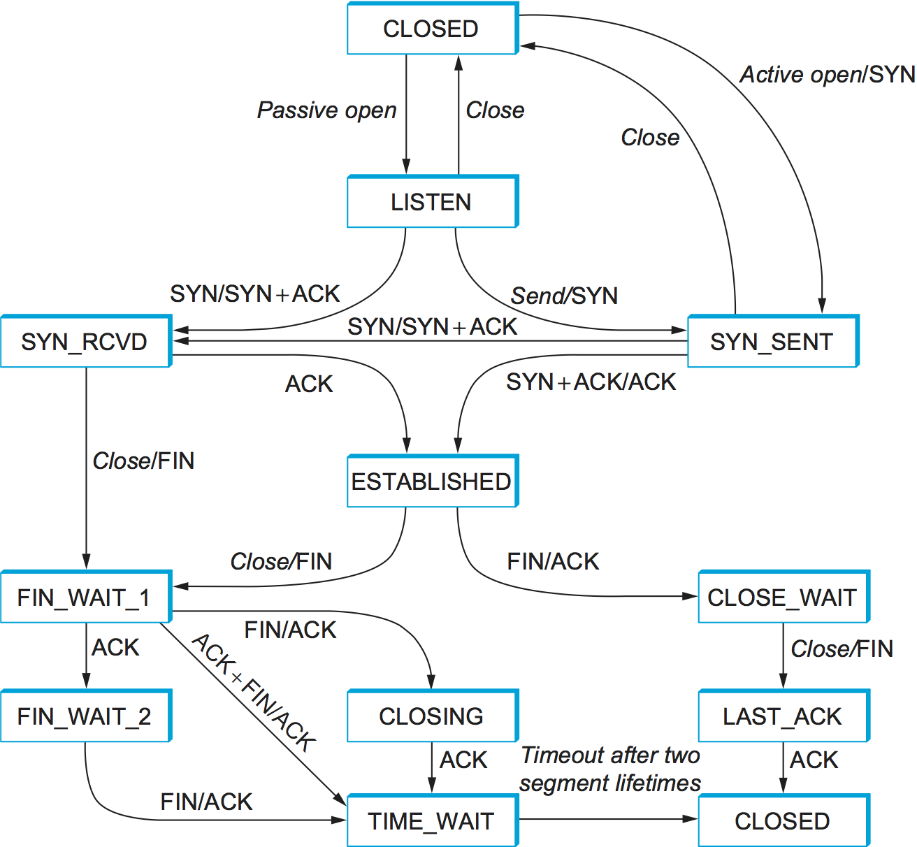
Figure 131. TCP state-transition diagram.
TCP’s state-transition diagram is fairly easy to understand. Each box
denotes a state that one end of a TCP connection can find itself in. All
connections start in the CLOSED state. As the connection progresses, the
connection moves from state to state according to the arcs. Each arc is
labeled with a tag of the form event/action. Thus, if a connection is
in the LISTEN state and a SYN segment arrives (i.e., a segment with the
SYN flag set), the connection makes a transition to the SYN_RCVD
state and takes the action of replying with an ACK+SYN segment.
Notice that two kinds of events trigger a state transition: (1) a segment arrives from the peer (e.g., the event on the arc from LISTEN to SYN_RCVD), or (2) the local application process invokes an operation on TCP (e.g., the active open event on the arc from CLOSED to SYN_SENT). In other words, TCP’s state-transition diagram effectively defines the semantics of both its peer-to-peer interface and its service interface. The syntax of these two interfaces is given by the segment format (as illustrated in Figure 128) and by some application programming interface, such as the socket API, respectively.
Now let’s trace the typical transitions taken through the diagram in Figure 131. Keep in mind that at each end of the connection, TCP makes different transitions from state to state. When opening a connection, the server first invokes a passive open operation on TCP, which causes TCP to move to the LISTEN state. At some later time, the client does an active open, which causes its end of the connection to send a SYN segment to the server and to move to the SYN_SENT state. When the SYN segment arrives at the server, it moves to the SYN_RCVD state and responds with a SYN+ACK segment. The arrival of this segment causes the client to move to the ESTABLISHED state and to send an ACK back to the server. When this ACK arrives, the server finally moves to the ESTABLISHED state. In other words, we have just traced the three-way handshake.
There are three things to notice about the connection establishment half
of the state-transition diagram. First, if the client’s ACK to the
server is lost, corresponding to the third leg of the three-way
handshake, then the connection still functions correctly. This is
because the client side is already in the ESTABLISHED state, so the
local application process can start sending data to the other end. Each
of these data segments will have the ACK flag set, and the correct
value in the Acknowledgement field, so the server will move to the
ESTABLISHED state when the first data segment arrives. This is actually
an important point about TCP—every segment reports what sequence number
the sender is expecting to see next, even if this repeats the same
sequence number contained in one or more previous segments.
The second thing to notice about the state-transition diagram is that there is a funny transition out of the LISTEN state whenever the local process invokes a send operation on TCP. That is, it is possible for a passive participant to identify both ends of the connection (i.e., itself and the remote participant that it is willing to have connect to it), and then for it to change its mind about waiting for the other side and instead actively establish the connection. To the best of our knowledge, this is a feature of TCP that no application process actually takes advantage of.
The final thing to notice about the diagram is the arcs that are not shown. Specifically, most of the states that involve sending a segment to the other side also schedule a timeout that eventually causes the segment to be resent if the expected response does not happen. These retransmissions are not depicted in the state-transition diagram. If after several tries the expected response does not arrive, TCP gives up and returns to the CLOSED state.
Turning our attention now to the process of terminating a connection, the important thing to keep in mind is that the application process on both sides of the connection must independently close its half of the connection. If only one side closes the connection, then this means it has no more data to send, but it is still available to receive data from the other side. This complicates the state-transition diagram because it must account for the possibility that the two sides invoke the close operator at the same time, as well as the possibility that first one side invokes close and then, at some later time, the other side invokes close. Thus, on any one side there are three combinations of transitions that get a connection from the ESTABLISHED state to the CLOSED state:
This side closes first: ESTABLISHED \(\rightarrow\) FIN_WAIT_1 \(\rightarrow\) FIN_WAIT_2 \(\rightarrow\) TIME_WAIT \(\rightarrow\) CLOSED.
The other side closes first: ESTABLISHED \(\rightarrow\) CLOSE_WAIT \(\rightarrow\) LAST_ACK \(\rightarrow\) CLOSED.
Both sides close at the same time: ESTABLISHED \(\rightarrow\) FIN_WAIT_1 \(\rightarrow\) CLOSING \(\rightarrow\) TIME_WAIT \(\rightarrow\) CLOSED.
There is actually a fourth, although rare, sequence of transitions that leads to the CLOSED state; it follows the arc from FIN_WAIT_1 to TIME_WAIT. We leave it as an exercise for you to figure out what combination of circumstances leads to this fourth possibility.
The main thing to recognize about connection teardown is that a connection in the TIME_WAIT state cannot move to the CLOSED state until it has waited for two times the maximum amount of time an IP datagram might live in the Internet (i.e., 120 seconds). The reason for this is that, while the local side of the connection has sent an ACK in response to the other side’s FIN segment, it does not know that the ACK was successfully delivered. As a consequence, the other side might retransmit its FIN segment, and this second FIN segment might be delayed in the network. If the connection were allowed to move directly to the CLOSED state, then another pair of application processes might come along and open the same connection (i.e., use the same pair of port numbers), and the delayed FIN segment from the earlier incarnation of the connection would immediately initiate the termination of the later incarnation of that connection.
5.2.4 Sliding Window Revisited
We are now ready to discuss TCP’s variant of the sliding window
algorithm, which serves several purposes: (1) it guarantees the reliable
delivery of data, (2) it ensures that data is delivered in order, and
(3) it enforces flow control between the sender and the receiver. TCP’s
use of the sliding window algorithm is the same as at the link level in
the case of the first two of these three functions. Where TCP differs
from the link-level algorithm is that it folds the flow-control function
in as well. In particular, rather than having a fixed-size sliding
window, the receiver advertises a window size to the sender. This is
done using the AdvertisedWindow field in the TCP header. The sender
is then limited to having no more than a value of AdvertisedWindow
bytes of unacknowledged data at any given time. The receiver selects a
suitable value for AdvertisedWindow based on the amount of memory
allocated to the connection for the purpose of buffering data. The idea
is to keep the sender from over-running the receiver’s buffer. We
discuss this at greater length below.
Reliable and Ordered Delivery
To see how the sending and receiving sides of TCP interact with each other to implement reliable and ordered delivery, consider the situation illustrated in Figure 132. TCP on the sending side maintains a send buffer. This buffer is used to store data that has been sent but not yet acknowledged, as well as data that has been written by the sending application but not transmitted. On the receiving side, TCP maintains a receive buffer. This buffer holds data that arrives out of order, as well as data that is in the correct order (i.e., there are no missing bytes earlier in the stream) but that the application process has not yet had the chance to read.

Figure 132. Relationship between TCP send buffer (a) and receive buffer (b).
To make the following discussion simpler to follow, we initially ignore the fact that both the buffers and the sequence numbers are of some finite size and hence will eventually wrap around. Also, we do not distinguish between a pointer into a buffer where a particular byte of data is stored and the sequence number for that byte.
Looking first at the sending side, three pointers are maintained into
the send buffer, each with an obvious meaning: LastByteAcked,
LastByteSent, and LastByteWritten. Clearly,
LastByteAcked <= LastByteSent
since the receiver cannot have acknowledged a byte that has not yet been sent, and
LastByteSent <= LastByteWritten
since TCP cannot send a byte that the application process has not yet
written. Also note that none of the bytes to the left of
LastByteAcked need to be saved in the buffer because they have
already been acknowledged, and none of the bytes to the right of
LastByteWritten need to be buffered because they have not yet been
generated.
A similar set of pointers (sequence numbers) are maintained on the
receiving side: LastByteRead, NextByteExpected, and
LastByteRcvd. The inequalities are a little less intuitive, however,
because of the problem of out-of-order delivery. The first relationship
LastByteRead < NextByteExpected
is true because a byte cannot be read by the application until it is
received and all preceding bytes have also been received.
NextByteExpected points to the byte immediately after the latest
byte to meet this criterion. Second,
NextByteExpected <= LastByteRcvd + 1
since, if data has arrived in order, NextByteExpected points to the
byte after LastByteRcvd, whereas if data has arrived out of order,
then NextByteExpected points to the start of the first gap in the
data, as in Figure 132. Note that bytes to the left of
LastByteRead need not be buffered because they have already been
read by the local application process, and bytes to the right of
LastByteRcvd need not be buffered because they have not yet arrived.
Flow Control
Most of the above discussion is similar to that found in the standard sliding window algorithm; the only real difference is that this time we elaborated on the fact that the sending and receiving application processes are filling and emptying their local buffer, respectively. (The earlier discussion glossed over the fact that data arriving from an upstream node was filling the send buffer and data being transmitted to a downstream node was emptying the receive buffer.)
You should make sure you understand this much before proceeding because
now comes the point where the two algorithms differ more significantly.
In what follows, we reintroduce the fact that both buffers are of some
finite size, denoted MaxSendBuffer and MaxRcvBuffer, although we
don’t worry about the details of how they are implemented. In other
words, we are only interested in the number of bytes being buffered, not
in where those bytes are actually stored.
Recall that in a sliding window protocol, the size of the window sets the amount of data that can be sent without waiting for acknowledgment from the receiver. Thus, the receiver throttles the sender by advertising a window that is no larger than the amount of data that it can buffer. Observe that TCP on the receive side must keep
LastByteRcvd - LastByteRead <= MaxRcvBuffer
to avoid overflowing its buffer. It therefore advertises a window size of
AdvertisedWindow = MaxRcvBuffer - ((NextByteExpected - 1) - LastByteRead)
which represents the amount of free space remaining in its buffer. As
data arrives, the receiver acknowledges it as long as all the preceding
bytes have also arrived. In addition, LastByteRcvd moves to the
right (is incremented), meaning that the advertised window potentially
shrinks. Whether or not it shrinks depends on how fast the local
application process is consuming data. If the local process is reading
data just as fast as it arrives (causing LastByteRead to be
incremented at the same rate as LastByteRcvd), then the advertised
window stays open (i.e., AdvertisedWindow = MaxRcvBuffer). If,
however, the receiving process falls behind, perhaps because it performs
a very expensive operation on each byte of data that it reads, then the
advertised window grows smaller with every segment that arrives, until
it eventually goes to 0.
TCP on the send side must then adhere to the advertised window it gets from the receiver. This means that at any given time, it must ensure that
LastByteSent - LastByteAcked <= AdvertisedWindow
Said another way, the sender computes an effective window that limits how much data it can send:
EffectiveWindow = AdvertisedWindow - (LastByteSent - LastByteAcked)
Clearly, EffectiveWindow must be greater than 0 before the source
can send more data. It is possible, therefore, that a segment arrives
acknowledging x bytes, thereby allowing the sender to increment
LastByteAcked by x, but because the receiving process was not
reading any data, the advertised window is now x bytes smaller than the
time before. In such a situation, the sender would be able to free
buffer space, but not to send any more data.
All the while this is going on, the send side must also make sure that the local application process does not overflow the send buffer—that is,
LastByteWritten - LastByteAcked <= MaxSendBuffer
If the sending process tries to write y bytes to TCP, but
(LastByteWritten - LastByteAcked) + y > MaxSendBuffer
then TCP blocks the sending process and does not allow it to generate more data.
It is now possible to understand how a slow receiving process ultimately
stops a fast sending process. First, the receive buffer fills up, which
means the advertised window shrinks to 0. An advertised window of 0
means that the sending side cannot transmit any data, even though data
it has previously sent has been successfully acknowledged. Finally, not
being able to transmit any data means that the send buffer fills up,
which ultimately causes TCP to block the sending process. As soon as the
receiving process starts to read data again, the receive-side TCP is
able to open its window back up, which allows the send-side TCP to
transmit data out of its buffer. When this data is eventually
acknowledged, LastByteAcked is incremented, the buffer space holding
this acknowledged data becomes free, and the sending process is
unblocked and allowed to proceed.
There is only one remaining detail that must be resolved—how does the
sending side know that the advertised window is no longer 0? As
mentioned above, TCP always sends a segment in response to a received
data segment, and this response contains the latest values for the
Acknowledge and AdvertisedWindow fields, even if these values
have not changed since the last time they were sent. The problem is
this. Once the receive side has advertised a window size of 0, the
sender is not permitted to send any more data, which means it has no way
to discover that the advertised window is no longer 0 at some time in
the future. TCP on the receive side does not spontaneously send nondata
segments; it only sends them in response to an arriving data segment.
TCP deals with this situation as follows. Whenever the other side advertises a window size of 0, the sending side persists in sending a segment with 1 byte of data every so often. It knows that this data will probably not be accepted, but it tries anyway, because each of these 1-byte segments triggers a response that contains the current advertised window. Eventually, one of these 1-byte probes triggers a response that reports a nonzero advertised window.
Note that these 1-byte messages are called Zero Window Probes and in practice they are sent every 5 to 60 seconds. As for what single byte of data to send in the probe: it’s the next byte of actual data just outside the window. (It has to be real data in case it’s accepted by the receiver.)
Key Takeaway
Note that the reason the sending side periodically sends this probe segment is that TCP is designed to make the receive side as simple as possible—it simply responds to segments from the sender, and it never initiates any activity on its own. This is an example of a well-recognized (although not universally applied) protocol design rule, which, for lack of a better name, we call the smart sender/ dumb receiver rule. Recall that we saw another example of this rule when we discussed the use of NAKs in sliding window algorithm. [Next]
Protecting Against Wraparound
This subsection and the next consider the size of the SequenceNum
and AdvertisedWindow fields and the implications of their sizes on
TCP’s correctness and performance. TCP’s SequenceNum field is
32 bits long, and its AdvertisedWindow field is 16 bits long,
meaning that TCP has easily satisfied the requirement of the sliding
window algorithm that the sequence number space be twice as big as the
window size: 232 >> 2 × 216. However, this
requirement is not the interesting thing about these two fields.
Consider each field in turn.
The relevance of the 32-bit sequence number space is that the sequence number used on a given connection might wrap around—a byte with sequence number S could be sent at one time, and then at a later time a second byte with the same sequence number S might be sent. Once again, we assume that packets cannot survive in the Internet for longer than the recommended MSL. Thus, we currently need to make sure that the sequence number does not wrap around within a 120-second period of time. Whether or not this happens depends on how fast data can be transmitted over the Internet—that is, how fast the 32-bit sequence number space can be consumed. (This discussion assumes that we are trying to consume the sequence number space as fast as possible, but of course we will be if we are doing our job of keeping the pipe full.) Table 22 shows how long it takes for the sequence number to wrap around on networks with various bandwidths.
Bandwidth |
Time until Wraparound |
|---|---|
T1 (1.5 Mbps) |
6.4 hours |
T3 (45 Mbps) |
13 minutes |
Fast Ethernet (100 Mbps) |
6 minutes |
OC-3 (155 Mbps) |
4 minutes |
OC-48 (2.5 Gbps) |
14 seconds |
OC-192 (10 Gbps) |
3 seconds |
10GigE (10 Gbps) |
3 seconds |
As you can see, the 32-bit sequence number space is adequate at modest bandwidths, but given that OC-192 links are now common in the Internet backbone, and that most servers now come with 10Gig Ethernet (or 10 Gbps) interfaces, we’re now well-past the point where 32 bits is too small. Fortunately, the IETF has worked out an extension to TCP that effectively extends the sequence number space to protect against the sequence number wrapping around. This and related extensions are described in a later section.
Keeping the Pipe Full
The relevance of the 16-bit AdvertisedWindow field is that it must
be big enough to allow the sender to keep the pipe full. Clearly, the
receiver is free to not open the window as large as the
AdvertisedWindow field allows; we are interested in the situation in
which the receiver has enough buffer space to handle as much data as the
largest possible AdvertisedWindow allows.
In this case, it is not just the network bandwidth but the delay x
bandwidth product that dictates how big the AdvertisedWindow field
needs to be—the window needs to be opened far enough to allow a full
delay × bandwidth product’s worth of data to be transmitted. Assuming an
RTT of 100 ms (a typical number for a cross-country connection in the
United States), Table 23 gives the delay × bandwidth
product for several network technologies.
Bandwidth |
Delay × Bandwidth Product |
|---|---|
T1 (1.5 Mbps) |
18 KB |
T3 (45 Mbps) |
549 KB |
Fast Ethernet (100 Mbps) |
1.2 MB |
OC-3 (155 Mbps) |
1.8 MB |
OC-48 (2.5 Gbps) |
29.6 MB |
OC-192 (10 Gbps) |
118.4 MB |
10GigE (10 Gbps) |
118.4 MB |
As you can see, TCP’s AdvertisedWindow field is in even worse shape
than its SequenceNum field—it is not big enough to handle even a T3
connection across the continental United States, since a 16-bit field
allows us to advertise a window of only 64 KB. The very same TCP
extension mentioned above provides a mechanism for effectively
increasing the size of the advertised window.
5.2.5 Triggering Transmission
We next consider a surprisingly subtle issue: how TCP decides to transmit a segment. As described earlier, TCP supports a byte-stream abstraction; that is, application programs write bytes into the stream, and it is up to TCP to decide that it has enough bytes to send a segment. What factors govern this decision?
If we ignore the possibility of flow control—that is, we assume the
window is wide open, as would be the case when a connection first
starts—then TCP has three mechanisms to trigger the transmission of a
segment. First, TCP maintains a variable, typically called the maximum
segment size (MSS), and it sends a segment as soon as it has
collected MSS bytes from the sending process. MSS is usually set
to the size of the largest segment TCP can send without causing the
local IP to fragment. That is, MSS is set to the maximum
transmission unit (MTU) of the directly connected network, minus the
size of the TCP and IP headers. The second thing that triggers TCP to
transmit a segment is that the sending process has explicitly asked it
to do so. Specifically, TCP supports a push operation, and the sending
process invokes this operation to effectively flush the buffer of unsent
bytes. The final trigger for transmitting a segment is that a timer
fires; the resulting segment contains as many bytes as are currently
buffered for transmission. However, as we will soon see, this “timer”
isn’t exactly what you expect.
Silly Window Syndrome
Of course, we can’t just ignore flow control, which plays an obvious
role in throttling the sender. If the sender has MSS bytes of data
to send and the window is open at least that much, then the sender
transmits a full segment. Suppose, however, that the sender is
accumulating bytes to send, but the window is currently closed. Now
suppose an ACK arrives that effectively opens the window enough for the
sender to transmit, say, MSS/2 bytes. Should the sender transmit a
half-full segment or wait for the window to open to a full MSS? The
original specification was silent on this point, and early
implementations of TCP decided to go ahead and transmit a half-full
segment. After all, there is no telling how long it will be before the
window opens further.
It turns out that the strategy of aggressively taking advantage of any
available window leads to a situation now known as the silly window
syndrome. Figure 133 helps visualize what
happens. If you think of a TCP stream as a conveyor belt with “full”
containers (data segments) going in one direction and empty containers
(ACKs) going in the reverse direction, then MSS-sized segments
correspond to large containers and 1-byte segments correspond to very
small containers. As long as the sender is sending MSS-sized
segments and the receiver ACKs at least one MSS of data at a time,
everything is good (Figure 133(a)). But,
what if the receiver has to reduce the window, so that at some time
the sender can’t send a full MSS of data? If the sender
aggressively fills a smaller-than-MSS empty container as soon as
it arrives, then the receiver will ACK that smaller number of bytes,
and hence the small container introduced into the system remains in
the system indefinitely. That is, it is immediately filled and
emptied at each end and is never coalesced with adjacent containers to
create larger containers, as in Figure 133(b). This scenario was discovered when early
implementations of TCP regularly found themselves filling the network
with tiny segments.
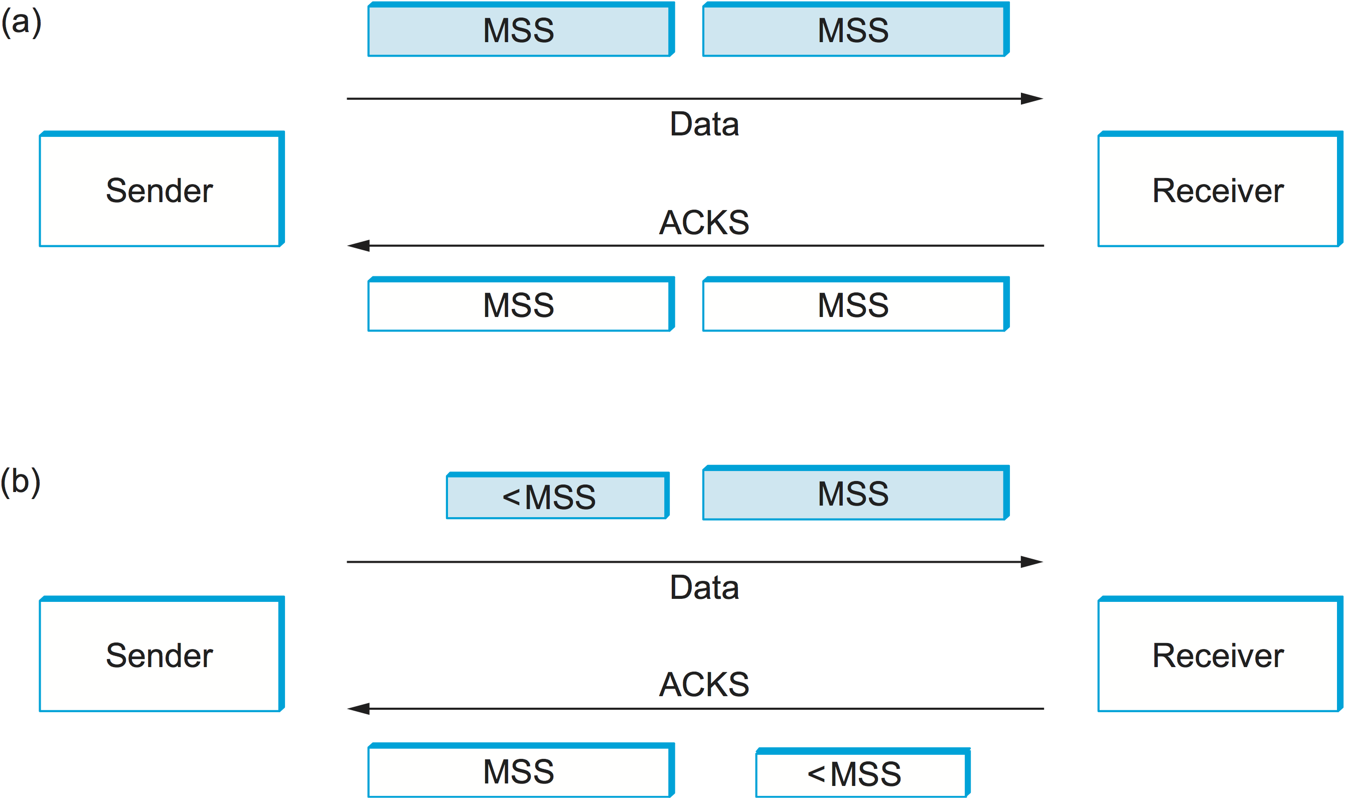
Figure 133. Silly window syndrome. (a) As long as the sender sends MSS-sized segments and the receiver ACKs one MSS at a time, the system works smoothly. (b) As soon as the sender sends less than one MSS, or the receiver ACKs less than one MSS, a small “container” enters the system and continues to circulate.
Note that the silly window syndrome is only a problem when either the
sender transmits a small segment or the receiver opens the window a
small amount. If neither of these happens, then the small container is
never introduced into the stream. It’s not possible to outlaw sending
small segments; for example, the application might do a push after
sending a single byte. It is possible, however, to keep the receiver
from introducing a small container (i.e., a small open window). The rule
is that after advertising a zero window the receiver must wait for space
equal to an MSS before it advertises an open window.
Since we can’t eliminate the possibility of a small container being introduced into the stream, we also need mechanisms to coalesce them. The receiver can do this by delaying ACKs—sending one combined ACK rather than multiple smaller ones—but this is only a partial solution because the receiver has no way of knowing how long it is safe to delay waiting either for another segment to arrive or for the application to read more data (thus opening the window). The ultimate solution falls to the sender, which brings us back to our original issue: When does the TCP sender decide to transmit a segment?
Nagle’s Algorithm
Returning to the TCP sender, if there is data to send but the window is
open less than MSS, then we may want to wait some amount of time
before sending the available data, but the question is how long? If we
wait too long, then we hurt interactive applications like Telnet. If we
don’t wait long enough, then we risk sending a bunch of tiny packets and
falling into the silly window syndrome. The answer is to introduce a
timer and to transmit when the timer expires.
While we could use a clock-based timer—for example, one that fires every 100 ms—Nagle introduced an elegant self-clocking solution. The idea is that as long as TCP has any data in flight, the sender will eventually receive an ACK. This ACK can be treated like a timer firing, triggering the transmission of more data. Nagle’s algorithm provides a simple, unified rule for deciding when to transmit:
When the application produces data to send
    if both the available data and the window >= MSS
        send a full segment
    else
        if there is unACKed data in flight
            buffer the new data until an ACK arrives
        else
            send all the new data now
In other words, it’s always OK to send a full segment if the window
allows. It’s also all right to immediately send a small amount of data
if there are currently no segments in transit, but if there is anything
in flight the sender must wait for an ACK before transmitting the next
segment. Thus, an interactive application like Telnet that continually
writes one byte at a time will send data at a rate of one segment per
RTT. Some segments will contain a single byte, while others will contain
as many bytes as the user was able to type in one round-trip time.
Because some applications cannot afford such a delay for each write it
does to a TCP connection, the socket interface allows the application to
turn off Nagle’s algorithm by setting the TCP_NODELAY option.
Setting this option means that data is transmitted as soon as possible.
5.2.6 Adaptive Retransmission
Because TCP guarantees the reliable delivery of data, it retransmits each segment if an ACK is not received in a certain period of time. TCP sets this timeout as a function of the RTT it expects between the two ends of the connection. Unfortunately, given the range of possible RTTs between any pair of hosts in the Internet, as well as the variation in RTT between the same two hosts over time, choosing an appropriate timeout value is not that easy. To address this problem, TCP uses an adaptive retransmission mechanism. We now describe this mechanism and how it has evolved over time as the Internet community has gained more experience using TCP.
Original Algorithm
We begin with a simple algorithm for computing a timeout value between a pair of hosts. This is the algorithm that was originally described in the TCP specification—and the following description presents it in those terms—but it could be used by any end-to-end protocol.
The idea is to keep a running average of the RTT and then to compute
the timeout as a function of this RTT. Specifically, every time TCP
sends a data segment, it records the time. When an ACK for that
segment arrives, TCP reads the time again, and then takes the
difference between these two times as a SampleRTT. TCP then
computes an EstimatedRTT as a weighted average between the
previous estimate and this new sample. That is,
EstimatedRTT = alpha x EstimatedRTT + (1 - alpha) x SampleRTT
The parameter alpha is selected to smooth the
EstimatedRTT. A small alpha tracks changes in the RTT but is
perhaps too heavily influenced by temporary fluctuations. On the other
hand, a large alpha is more stable but perhaps not quick enough to
adapt to real changes. The original TCP specification recommended a
setting of alpha between 0.8 and 0.9. TCP then uses
EstimatedRTT to compute the timeout in a rather conservative way:
TimeOut = 2 x EstimatedRTT
Karn/Partridge Algorithm
After several years of use on the Internet, a rather obvious flaw was
discovered in this simple algorithm. The problem was that an ACK does
not really acknowledge a transmission; it actually acknowledges the
receipt of data. In other words, whenever a segment is retransmitted
and then an ACK arrives at the sender, it is impossible to determine
if this ACK should be associated with the first or the second
transmission of the segment for the purpose of measuring the sample
RTT. It is necessary to know which transmission to associate it with
so as to compute an accurate SampleRTT. As illustrated in
Figure 134, if you assume that the ACK is for
the original transmission but it was really for the second, then the
SampleRTT is too large (a); if you assume that the ACK is for the
second transmission but it was actually for the first, then the
SampleRTT is too small (b).
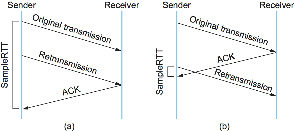
Figure 134. Associating the ACK with (a) original transmission versus (b) retransmission.
The solution, which was proposed in 1987, is surprisingly simple.
Whenever TCP retransmits a segment, it stops taking samples of the RTT;
it only measures SampleRTT for segments that have been sent only
once. This solution is known as the Karn/Partridge algorithm, after its
inventors. Their proposed fix also includes a second small change to
TCP’s timeout mechanism. Each time TCP retransmits, it sets the next
timeout to be twice the last timeout, rather than basing it on the last
EstimatedRTT. That is, Karn and Partridge proposed that TCP use
exponential backoff, similar to what the Ethernet does. The motivation
for using exponential backoff is simple: Congestion is the most likely
cause of lost segments, meaning that the TCP source should not react too
aggressively to a timeout. In fact, the more times the connection times
out, the more cautious the source should become. We will see this idea
again, embodied in a much more sophisticated mechanism, in the next
chapter.
Jacobson/Karels Algorithm
The Karn/Partridge algorithm was introduced at a time when the Internet was suffering from high levels of network congestion. Their approach was designed to fix some of the causes of that congestion, but, although it was an improvement, the congestion was not eliminated. The following year (1988), two other researchers—Jacobson and Karels—proposed a more drastic change to TCP to battle congestion. The bulk of that proposed change is described in the next chapter. Here, we focus on the aspect of that proposal that is related to deciding when to time out and retransmit a segment.
As an aside, it should be clear how the timeout mechanism is related to congestion—if you time out too soon, you may unnecessarily retransmit a segment, which only adds to the load on the network. The other reason for needing an accurate timeout value is that a timeout is taken to imply congestion, which triggers a congestion-control mechanism. Finally, note that there is nothing about the Jacobson/Karels timeout computation that is specific to TCP. It could be used by any end-to-end protocol.
The main problem with the original computation is that it does not take
the variance of the sample RTTs into account. Intuitively, if the
variation among samples is small, then the EstimatedRTT can be
better trusted and there is no reason for multiplying this estimate by 2
to compute the timeout. On the other hand, a large variance in the
samples suggests that the timeout value should not be too tightly
coupled to the EstimatedRTT.
In the new approach, the sender measures a new SampleRTT as before.
It then folds this new sample into the timeout calculation as follows:
Difference = SampleRTT - EstimatedRTT
EstimatedRTT = EstimatedRTT + ( delta x Difference)
Deviation = Deviation + delta (|Difference| - Deviation)
where delta is between 0 and 1. That is, we calculate both the
mean RTT and the variation in that mean.
TCP then computes the timeout value as a function of both
EstimatedRTT and Deviation as follows:
TimeOut = mu x EstimatedRTT + phi x Deviation
where based on experience, mu is typically set to 1 and phi is
set to 4. Thus, when the variance is small, TimeOut is close to
EstimatedRTT; a large variance causes the Deviation term to
dominate the calculation.
Implementation
There are two items of note regarding the implementation of timeouts in
TCP. The first is that it is possible to implement the calculation for
EstimatedRTT and Deviation without using floating-point
arithmetic. Instead, the whole calculation is scaled by 2n,
with delta selected to be 1/2n. This allows us to do integer
arithmetic, implementing multiplication and division using shifts,
thereby achieving higher performance. The resulting calculation is given
by the following code fragment, where n=3
(i.e., delta = 1/8). Note that EstimatedRTT and Deviation are
stored in their scaled-up forms, while the value of SampleRTT at the
start of the code and of TimeOut at the end are real, unscaled
values. If you find the code hard to follow, you might want to try
plugging some real numbers into it and verifying that it gives the same
results as the equations above.
{
    SampleRTT -= (EstimatedRTT >> 3);
    EstimatedRTT += SampleRTT;
    if (SampleRTT < 0)
        SampleRTT = -SampleRTT;
    SampleRTT -= (Deviation >> 3);
    Deviation += SampleRTT;
    TimeOut = (EstimatedRTT >> 3) + (Deviation >> 1);
}
The second point of note is that the Jacobson/Karels algorithm is only as good as the clock used to read the current time. On typical Unix implementations at the time, the clock granularity was as large as 500 ms, which is significantly larger than the average cross-country RTT of somewhere between 100 and 200 ms. To make matters worse, the Unix implementation of TCP only checked to see if a timeout should happen every time this 500-ms clock ticked and would only take a sample of the round-trip time once per RTT. The combination of these two factors could mean that a timeout would happen 1 second after the segment was transmitted. Once again, the extensions to TCP include a mechanism that makes this RTT calculation a bit more precise.
All of the retransmission algorithms we have discussed are based on acknowledgment timeouts, which indicate that a segment has probably been lost. Note that a timeout does not, however, tell the sender whether any segments it sent after the lost segment were successfully received. This is because TCP acknowledgments are cumulative; they identify only the last segment that was received without any preceding gaps. The reception of segments that occur after a gap grows more frequent as faster networks lead to larger windows. If ACKs also told the sender which subsequent segments, if any, had been received, then the sender could be more intelligent about which segments it retransmits, draw better conclusions about the state of congestion, and make better RTT estimates. A TCP extension supporting this is described in a later section.
Key Takeaway
There is one other point to make about computing timeouts. It is a surprisingly tricky business, so much so, that there is an entire RFC dedicated to the topic: RFC 6298. The takeaway is that sometimes fully specifying a protocol involves so much minutiae that the line between specification and implementation becomes blurred. That has happened more than once with TCP, causing some to argue that “the implementation is the specification.” But that’s not necessarily a bad thing as long as the reference implementation is available as open source software. More generally, the industry is seeing open source software grow in importance as open standards recede in importance. [Next]
5.2.7 Record Boundaries
Since TCP is a byte-stream protocol, the number of bytes written by the sender are not necessarily the same as the number of bytes read by the receiver. For example, the application might write 8 bytes, then 2 bytes, then 20 bytes to a TCP connection, while on the receiving side the application reads 5 bytes at a time inside a loop that iterates 6 times. TCP does not interject record boundaries between the 8th and 9th bytes, nor between the 10th and 11th bytes. This is in contrast to a message-oriented protocol, such as UDP, in which the message that is sent is exactly the same length as the message that is received.
Even though TCP is a byte-stream protocol, it has two different features that can be used by the sender to insert record boundaries into this byte stream, thereby informing the receiver how to break the stream of bytes into records. (Being able to mark record boundaries is useful, for example, in many database applications.) Both of these features were originally included in TCP for completely different reasons; they have only come to be used for this purpose over time.
The first mechanism is the urgent data feature, as implemented by the
URG flag and the UrgPtr field in the TCP header. Originally, the
urgent data mechanism was designed to allow the sending application to
send out-of-band data to its peer. By “out of band” we mean data that
is separate from the normal flow of data (e.g., a command to interrupt
an operation already under way). This out-of-band data was identified in
the segment using the UrgPtr field and was to be delivered to the
receiving process as soon as it arrived, even if that meant delivering
it before data with an earlier sequence number. Over time, however, this
feature has not been used, so instead of signifying “urgent” data, it
has come to be used to signify “special” data, such as a record marker.
This use has developed because, as with the push operation, TCP on the
receiving side must inform the application that urgent data has arrived.
That is, the urgent data in itself is not important. It is the fact that
the sending process can effectively send a signal to the receiver that
is important.
The second mechanism for inserting end-of-record markers into a byte is the push operation. Originally, this mechanism was designed to allow the sending process to tell TCP that it should send (flush) whatever bytes it had collected to its peer. The push operation can be used to implement record boundaries because the specification says that TCP must send whatever data it has buffered at the source when the application says push, and, optionally, TCP at the destination notifies the application whenever an incoming segment has the PUSH flag set. If the receiving side supports this option (the socket interface does not), then the push operation can be used to break the TCP stream into records.
Of course, the application program is always free to insert record boundaries without any assistance from TCP. For example, it can send a field that indicates the length of a record that is to follow, or it can insert its own record boundary markers into the data stream.
5.2.8 TCP Extensions
We have mentioned at four different points in this section that there
are now extensions to TCP that help to mitigate some problem that TCP
faced as the underlying network got faster. These extensions are
designed to have as small an impact on TCP as possible. In particular,
they are realized as options that can be added to the TCP header. (We
glossed over this point earlier, but the reason why the TCP header has a
HdrLen field is that the header can be of variable length; the
variable part of the TCP header contains the options that have been
added.) The significance of adding these extensions as options rather
than changing the core of the TCP header is that hosts can still
communicate using TCP even if they do not implement the options. Hosts
that do implement the optional extensions, however, can take advantage
of them. The two sides agree that they will use the options during TCP’s
connection establishment phase.
The first extension helps to improve TCP’s timeout mechanism. Instead of measuring the RTT using a coarse-grained event, TCP can read the actual system clock when it is about to send a segment, and put this time—think of it as a 32-bit timestamp—in the segment’s header. The receiver then echoes this timestamp back to the sender in its acknowledgment, and the sender subtracts this timestamp from the current time to measure the RTT. In essence, the timestamp option provides a convenient place for TCP to store the record of when a segment was transmitted; it stores the time in the segment itself. Note that the endpoints in the connection do not need synchronized clocks, since the timestamp is written and read at the same end of the connection.
The second extension addresses the problem of TCP’s 32-bit
SequenceNum field wrapping around too soon on a high-speed network.
Rather than define a new 64-bit sequence number field, TCP uses the
32-bit timestamp just described to effectively extend the sequence
number space. In other words, TCP decides whether to accept or reject a
segment based on a 64-bit identifier that has the SequenceNum field
in the low-order 32 bits and the timestamp in the high-order 32 bits.
Since the timestamp is always increasing, it serves to distinguish
between two different incarnations of the same sequence number. Note
that the timestamp is being used in this setting only to protect against
wraparound; it is not treated as part of the sequence number for the
purpose of ordering or acknowledging data.
The third extension allows TCP to advertise a larger window, thereby
allowing it to fill larger delay × bandwidth pipes that are made
possible by high-speed networks. This extension involves an option that
defines a scaling factor for the advertised window. That is, rather
than interpreting the number that appears in the AdvertisedWindow
field as indicating how many bytes the sender is allowed to have
unacknowledged, this option allows the two sides of TCP to agree that
the AdvertisedWindow field counts larger chunks (e.g., how many
16-byte units of data the sender can have unacknowledged). In other
words, the window scaling option specifies how many bits each side
should left-shift the AdvertisedWindow field before using its
contents to compute an effective window.
The fourth extension allows TCP to augment its cumulative acknowledgment
with selective acknowledgments of any additional segments that have been
received but aren’t contiguous with all previously received segments.
This is the selective acknowledgment, or SACK, option. When the SACK
option is used, the receiver continues to acknowledge segments
normally—the meaning of the Acknowledge field does not change—but it
also uses optional fields in the header to acknowledge any additional
blocks of received data. This allows the sender to retransmit just the
segments that are missing according to the selective acknowledgment.
Without SACK, there are only two reasonable strategies for a sender. The pessimistic strategy responds to a timeout by retransmitting not just the segment that timed out, but any segments transmitted subsequently. In effect, the pessimistic strategy assumes the worst: that all those segments were lost. The disadvantage of the pessimistic strategy is that it may unnecessarily retransmit segments that were successfully received the first time. The other strategy is the optimistic strategy, which responds to a timeout by retransmitting only the segment that timed out. In effect, the optimistic approach assumes the rosiest scenario: that only the one segment has been lost. The disadvantage of the optimistic strategy is that it is very slow, unnecessarily, when a series of consecutive segments has been lost, as might happen when there is congestion. It is slow because each segment’s loss is not discovered until the sender receives an ACK for its retransmission of the previous segment. So it consumes one RTT per segment until it has retransmitted all the segments in the lost series. With the SACK option, a better strategy is available to the sender: retransmit just the segments that fill the gaps between the segments that have been selectively acknowledged.
These extensions, by the way, are not the full story. We’ll see some more extensions in the next chapter when we look at how TCP handles congestion. The Internet Assigned Numbers Authority (IANA) keeps track of all the options that are defined for TCP (and for many other Internet protocols). See the references at the end of the chapter for a link to IANA’s protocol number registry.
5.2.9 Performance
Recall that Chapter 1 introduced the two quantitative metrics by which network performance is evaluated: latency and throughput. As mentioned in that discussion, these metrics are influenced not only by the underlying hardware (e.g., propagation delay and link bandwidth) but also by software overheads. Now that we have a complete software-based protocol graph available to us that includes alternative transport protocols, we can discuss how to meaningfully measure its performance. The importance of such measurements is that they represent the performance seen by application programs.
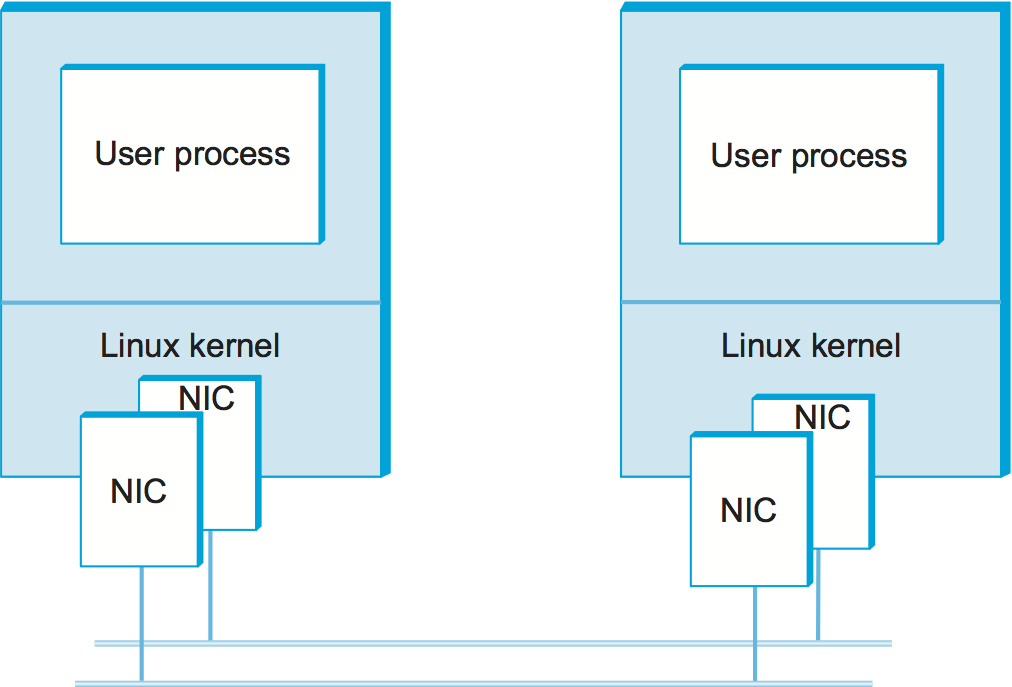
Figure 135. Measured system: Two Linux workstations and a pair of Gbps Ethernet links.
We begin, as any report of experimental results should, by describing our experimental method. This includes the apparatus used in the experiments; in this case, each workstation has a pair of dual CPU 2.4-GHz Xeon processors running Linux. In order to enable speeds above 1 Gbps, a pair of Ethernet adaptors (labeled NIC, for network interface card) are used on each machine. The Ethernet spans a single machine room so propagation is not an issue, making this a measure of processor/software overheads. A test program running on top of the socket interface simply tries to transfer data as quickly as possible from one machine to the other. Figure 135 illustrates the setup.
You may notice that this experimental setup is not especially bleeding edge in terms of the hardware or link speed. The point of this section is not to show how fast a particular protocol can run, but to illustrate the general methodology for measuring and reporting protocol performance.
The throughput test is performed for a variety of message sizes using a standard benchmarking tool called TTCP. The results of the throughput test are given in Figure 136. The key thing to notice in this graph is that throughput improves as the messages get larger. This makes sense—each message involves a certain amount of overhead, so a larger message means that this overhead is amortized over more bytes. The throughput curve flattens off above 1 KB, at which point the per-message overhead becomes insignificant when compared to the large number of bytes that the protocol stack has to process.
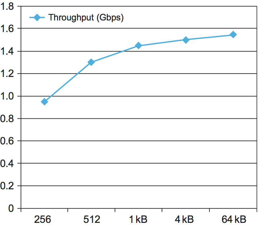
Figure 136. Measured throughput using TCP, for various message sizes.
It’s worth noting that the maximum throughput is less than 2 Gbps, the available link speed in this setup. Further testing and analysis of results would be needed to figure out where the bottleneck is (or if there is more than one). For example, looking at CPU load might give an indication of whether the CPU is the bottleneck or whether memory bandwidth, adaptor performance, or some other issue is to blame.
We also note that the network in this test is basically “perfect.” It has almost no delay or loss, so the only factors affecting performance are the TCP implementation and the workstation hardware and software. By contrast, most of the time we deal with networks that are far from perfect, notably our bandwidth-constrained, last-mile links and loss-prone wireless links. Before we can fully appreciate how these links affect TCP performance, we need to understand how TCP deals with congestion, which is the topic of the next chapter.
At various times in the history of networking, the steadily increasing speed of network links has threatened to run ahead of what could be delivered to applications. For example, a large research effort was begun in the United States in 1989 to build “gigabit networks,” where the goal was not only to build links and switches that could run at 1Gbps or higher but also to deliver that throughput all the way to a single application process. There were some real problems (e.g., network adaptors, workstation architectures, and operating systems all had to be designed with network-to-application throughput in mind) and also some perceived problems that turned out to be not so serious. High on the list of such problems was the concern that existing transport protocols, TCP in particular, might not be up to the challenge of gigabit operation.
As it turns out, TCP has done well keeping up with the increasing demands of high-speed networks and applications. One of the most important factors was the introduction of window scaling to deal with larger bandwidth-delay products. However, there is often a big difference between the theoretical performance of TCP and what is achieved in practice. Relatively simple problems like copying the data more times than necessary as it passes from network adaptor to application can drive down performance, as can insufficient buffer memory when the bandwidth-delay product is large. And the dynamics of TCP are complex enough (as will become even more apparent in the next chapter) that subtle interactions among network behavior, application behavior, and the TCP protocol itself can dramatically alter performance.
For our purposes, it’s worth noting that TCP continues to perform very well as network speeds increase, and when it runs up against some limit (normally related to congestion, increasing bandwidth-delay products, or both), researchers rush in to find solutions. We’ve seen some of those in this chapter, and we’ll see some more in the next.
5.2.10 Alternative Design Choices (SCTP, QUIC)
Although TCP has proven to be a robust protocol that satisfies the needs of a wide range of applications, the design space for transport protocols is quite large. TCP is by no means the only valid point in that design space. We conclude our discussion of TCP by considering alternative design choices. While we offer an explanation for why TCP’s designers made the choices they did, we observe that other protocols exist that have made other choices, and more such protocols may appear in the future.
First, we have suggested from the very first chapter of this book that there are at least two interesting classes of transport protocols: stream-oriented protocols like TCP and request/reply protocols like RPC. In other words, we have implicitly divided the design space in half and placed TCP squarely in the stream-oriented half of the world. We could further divide the stream-oriented protocols into two groups—reliable and unreliable—with the former containing TCP and the latter being more suitable for interactive video applications that would rather drop a frame than incur the delay associated with a retransmission.
This exercise in building a transport protocol taxonomy is interesting and could be continued in greater and greater detail, but the world isn’t as black and white as we might like. Consider the suitability of TCP as a transport protocol for request/reply applications, for example. TCP is a full-duplex protocol, so it would be easy to open a TCP connection between the client and server, send the request message in one direction, and send the reply message in the other direction. There are two complications, however. The first is that TCP is a byte-oriented protocol rather than a message-oriented protocol, and request/reply applications always deal with messages. (We explore the issue of bytes versus messages in greater detail in a moment.) The second complication is that in those situations where both the request message and the reply message fit in a single network packet, a well-designed request/reply protocol needs only two packets to implement the exchange, whereas TCP would need at least nine: three to establish the connection, two for the message exchange, and four to tear down the connection. Of course, if the request or reply messages are large enough to require multiple network packets (e.g., it might take 100 packets to send a 100,000-byte reply message), then the overhead of setting up and tearing down the connection is inconsequential. In other words, it isn’t always the case that a particular protocol cannot support a certain functionality; it’s sometimes the case that one design is more efficient than another under particular circumstances.
Second, as just suggested, you might question why TCP chose to provide a reliable byte-stream service rather than a reliable message-stream service; messages would be the natural choice for a database application that wants to exchange records. There are two answers to this question. The first is that a message-oriented protocol must, by definition, establish an upper bound on message sizes. After all, an infinitely long message is a byte stream. For any message size that a protocol selects, there will be applications that want to send larger messages, rendering the transport protocol useless and forcing the application to implement its own transport-like services. The second reason is that, while message-oriented protocols are definitely more appropriate for applications that want to send records to each other, you can easily insert record boundaries into a byte stream to implement this functionality.
A third decision made in the design of TCP is that it delivers bytes in order to the application. This means that it may hold onto bytes that were received out of order from the network, awaiting some missing bytes to fill a hole. This is enormously helpful for many applications but turns out to be quite unhelpful if the application is capable of processing data out of order. As a simple example, a Web page containing multiple embedded objects doesn’t need all the objects to be delivered in order before starting to display the page. In fact, there is a class of applications that would prefer to handle out-of-order data at the application layer, in return for getting data sooner when packets are dropped or misordered within the network. The desire to support such applications led to the creation of not one but two IETF standard transport protocols. The first of these was SCTP, the Stream Control Transmission Protocol. SCTP provides a partially ordered delivery service, rather than the strictly ordered service of TCP. (SCTP also makes some other design decisions that differ from TCP, including message orientation and support of multiple IP addresses for a single session.) More recently, the IETF has been standardizing a protocol optimized for Web traffic, known as QUIC. More on QUIC in a moment.
Fourth, TCP chose to implement explicit setup/teardown phases, but this is not required. In the case of connection setup, it would be possible to send all necessary connection parameters along with the first data message. TCP elected to take a more conservative approach that gives the receiver the opportunity to reject the connection before any data arrives. In the case of teardown, we could quietly close a connection that has been inactive for a long period of time, but this would complicate applications like remote login that want to keep a connection alive for weeks at a time; such applications would be forced to send out-of-band “keep alive” messages to keep the connection state at the other end from disappearing.
Finally, TCP is a window-based protocol, but this is not the only
possibility. The alternative is a rate-based design, in which the
receiver tells the sender the rate—expressed in either bytes or packets
per second—at which it is willing to accept incoming data. For example,
the receiver might inform the sender that it can accommodate 100 packets
a second. There is an interesting duality between windows and rate,
since the number of packets (bytes) in the window, divided by the RTT,
is exactly the rate. For example, a window size of 10 packets and a
100-ms RTT implies that the sender is allowed to transmit at a rate of
100 packets a second. It is by increasing or decreasing the advertised
window size that the receiver is effectively raising or lowering the
rate at which the sender can transmit. In TCP, this information is fed
back to the sender in the AdvertisedWindow field of the ACK for
every segment. One of the key issues in a rate-based protocol is how
often the desired rate—which may change over time—is relayed back to the
source: Is it for every packet, once per RTT, or only when the rate
changes? While we have just now considered window versus rate in the
context of flow control, it is an even more hotly contested issue in the
context of congestion control, which we will discuss in the next
chapter.
QUIC
QUIC originated at Google in 2012 and was subsequently developed as a proposed standard at the IETF. Unlike many other efforts to add to the set of transport protocols in the Internet, QUIC has achieved widespread deployment. As discussed further in Chapter 9, QUIC was motivated in large part by the challenges of matching the request/response semantics of HTTP to the stream-oriented nature of TCP. These issues have become more noticeable over time, due to factors such as the rise of high-latency wireless networks, the availability of multiple networks for a single device (e.g., Wi-Fi and cellular), and the increasing use of encrypted, authenticated connections on the Web (as discussed in Chapter 8). While a full description of QUIC is beyond our scope, some of the key design decisions are worth discussing.
If network latency is high—say 100 milliseconds or more—then a few RTTs can quickly add up to a visible annoyance for an end user. Establishing an HTTP session over TCP with Transport Layer Security (Section 8.5) would typically take at least three round trips (one for TCP session establishment and two for setting up the encryption parameters) before the first HTTP message could be sent. The designers of QUIC recognized that this delay—the direct result of a layered approach to protocol design—could be dramatically reduced if connection setup and the required security handshakes were combined and optimized for minimal round trips.
Note also how the presence of multiple network interfaces might affect the design. If your mobile phone loses its Wi-Fi connection and needs to switch to a cellular connection, that would typically require both a TCP timeout on one connection and a new series of handshakes on the other. Making the connection something that can persist over different network layer connections was another design goal for QUIC.
Finally, as noted above, the reliable byte stream model for TCP is a poor match to a Web page request, when many objects need to be fetched and page rendering could begin before they have all arrived. While one workaround for this would be to open multiple TCP connections in parallel, this approach (which was used in the early days of the Web) has its own set of drawbacks, notably on congestion control (see Chapter 6). Specifically, each connection runs its own congestion control loop, so the experience of congestion on one connection is not apparent to the other connections, and each connection tries to figure out the appropriate amount of bandwidth to consume on its own. QUIC introduced the idea of streams within a connection, so that objects could be delivered out-of-order while maintaining a holistic view of congestion across all the streams.
Interestingly, by the time QUIC emerged, many design decisions had been made that presented challenges for the deployment of a new transport protocol. Notably, many “middleboxes’’ such as NATs and firewalls (see Section 8.5) have enough understanding of the existing widespread transport protocols (TCP and UDP) that they can’t be relied upon to pass a new transport protocol. As a result, QUIC actually rides on top of UDP. In other words, it is a transport protocol running on top of a transport protocol. This is not as uncommon as our focus on layering might suggest, as the next two subsections also illustrate. This choice was made in the interests of making QUIC deployable on the Internet as it exists, and has been quite successful.
QUIC implements fast connection establishment with encryption and authentication in the first RTT. It provides a connection identifier that persists across changes in the underlying network. It supports the multiplexing of several streams onto a single transport connection, to avoid the head-of-line blocking that may arise when a single packet is dropped while other useful data continues to arrive. And it preserves (and in some ways improves on) the congestion avoidance properties of TCP, an important aspect of transport protocols that we return to in Chapter 6.
HTTP went through a number of versions (1.0, 1.1, 2.0, discussed in Section 9.1) in an effort to map its requirements more cleanly onto the capabilities of TCP. With the arrival of QUIC, HTTP/3 is now able to leverage a transport layer that was explicitly designed to meet the application requirements of the Web.
QUIC is a most interesting development in the world of transport protocols. Many of the limitations of TCP have been known for decades, but QUIC represents one of the most successful efforts to date to stake out a different point in the design space. Because QUIC was inspired by experience with HTTP and the Web—which arose long after TCP was well established in the Internet—it presents a fascinating case study in the unforeseen consequences of layered designs and in the evolution of the Internet.